
n-layer sphere: pointwise fields
The strain, stress and displacement at a point inside — and outside — an n-layer composite sphere, under an arbitrary remote loading, with perfect or imperfect interfaces.
Where layer_strain_average gives one tensor per layer, the pointwise API gives the field itself:
LayeredSphereFields(sphere, C₀)— solve the recurrence once;local_strain_strain_loc(sol, x)—with local_stress_strain_loc,local_strain_stress_loc,local_stress_stress_locfor a remote stress;local_strain,local_stress,local_displacement— the fields for one loading;get_layer(sphere, r; side)— which region a radius belongs to, and which limit is meant exactly on an interface.
TensTI{4,T,6}: six Walpole scalars and an axis, not an 81-component array.
using MeanFieldHomogenization
using TensND
using LinearAlgebra
using Printf
using Plots
gr()

default(; left_margin = 5Plots.mm, bottom_margin = 5Plots.mm)
Setup — a stiff core in a compliant ITZ shell
The classic three-phase model of a cement paste: a stiff aggregate, a compliant interfacial transition zone, and the matrix at infinity.
_stiff_Enu(E, ν) = TensISO{3}(3E / (3 * (1 - 2ν)), 2E / (2 * (1 + ν)))

const C₀ = _stiff_Enu(30.0, 0.3)      # matrix
const Cᵢ = _stiff_Enu(100.0, 0.2)     # core (aggregate)
const Cₛ = _stiff_Enu(10.0, 0.35)      # ITZ shell

const R = 1.0                          # core radius
const Rₛ = 1.5                         # shell outer radius

const sphere = LayeredSphere((R, Rₛ), (Cᵢ, Cₛ))
const sol = LayeredSphereFields(sphere, C₀)
LayeredSphereFields{Float64, 2, 3, LayeredSphere{Float64, 2, Tuple{TensND.TensISO{4, 3, Float64, 2}, TensND.TensISO{4, 3, Float64, 2}}, Tuple{PerfectInterface{Float64}, PerfectInterface{Float64}}}, TensND.TensISO{4, 3, Float64, 2}}(LayeredSphere{Float64} (2 layer(s), radii = (1.0, 1.5)), (74.99999999999999) 𝕁 + (23.076923076923077) 𝕂, ((55.555555555555564, 41.66666666666667), (11.111111111111109, 3.7037037037037033)), (24.999999999999996, 11.538461538461538), ((0.44234257061318083, 0.0), (1.6672912276958363, -1.224948657082656), (1.0, 1.027159236390792)), ((0.3545262663706544, -0.0012923628849353186, 0.0, 0.0), (2.0074018553266955, -0.003124393787755693, 1.0017092294567276, -0.5162635568179808), (1.0, 0.0, -1.7279627527107215, 0.3418816990365294)))Radial profiles under a hydrostatic far field
const εᵥ = 1.0
const ε∞_hyd = εᵥ * TensISO{3}(1.0)

"Radial and hoop stress at radius `r` under the remote loading `ε∞`."
function radial_hoop(sol, r, ε∞; side = :outer)
    σ = local_stress(sol, [r, 0.0, 0.0], ε∞; side)
    return σ[1, 1], σ[2, 2]              # e₁ is radial here, e₂ is a hoop axis
end

rs = range(1.0e-6, 4 * Rₛ; length = 600)
σrr_h = [radial_hoop(sol, r, ε∞_hyd)[1] for r in rs]
σθθ_h = [radial_hoop(sol, r, ε∞_hyd)[2] for r in rs]

σ_far = 3 * (30.0 / (3 * (1 - 2 * 0.3))) * εᵥ   # 3K₀ εᵥ

println("Hydrostatic far field, σ∞ᵢᵢ = 3K₀εᵥ = ", round(σ_far; digits = 4))
@printf "  %-9s  %12s  %12s\n" "r" "σ_rr" "σ_θθ"
for r in (0.5R, R, 0.5(R + Rₛ), Rₛ, 2Rₛ)
    σrr, σθθ = radial_hoop(sol, r, ε∞_hyd)
    @printf "  %-9.4f  %+12.6f  %+12.6f\n" r σrr σθθ
end
Hydrostatic far field, σ∞ᵢᵢ = 3K₀εᵥ = 75.0
r σ_rr σ_θθ
0.5000 +73.723762 +73.723762
1.0000 +73.723762 +46.502681
1.2500 +64.867837 +50.930643
1.5000 +60.953378 +82.023311
3.0000 +73.244172 +75.877914Continuity of the radial traction is a property of the solution, not something imposed on the plot — side = :inner and side = :outer are the two limits at an interface radius.
for r in (R, Rₛ)
    Δ = abs(
        radial_hoop(sol, r, ε∞_hyd; side = :outer)[1] -
            radial_hoop(sol, r, ε∞_hyd; side = :inner)[1]
    )
    @printf "  σ_rr continuity at r = %.2f :  Δ = %.3e\n" r Δ
end
σ_rr continuity at r = 1.00 : Δ = 2.842e-14
σ_rr continuity at r = 1.50 : Δ = 1.421e-14Radial profiles under a deviatoric far field
The deviatoric (
const ε∞_dev = Tens(diagm([0.0, 0.0, 1.0]))3×3 TensND.TensCanonical{2, 3, Float64, Tensors.SymmetricTensor{2, 3, Float64, 6}}:
0.0 0.0 0.0
0.0 0.0 0.0
0.0 0.0 1.0Note the two spellings of a point: a Cartesian vector, as here, or the three separate arguments (r, θ, φ). local_stress(sol, a, b, c, ε∞) is the SPHERICAL form — passing Cartesian components that way silently evaluates somewhere else entirely.
"σ in the meridian plane φ = 0, at colatitude θ, in the canonical basis."
σ_at(sol, r, θ, ε∞; side = :outer) =
    local_stress(sol, [r * sin(θ), 0.0, r * cos(θ)], ε∞; side)

σzz_pole = [σ_at(sol, r, 0.0, ε∞_dev)[3, 3] for r in rs]      # along the load axis
σzz_eq = [σ_at(sol, r, π / 2, ε∞_dev)[3, 3] for r in rs]      # perpendicular to it
600-element Vector{Float64}:
44.27049094354253
44.27010186153451
44.26893477085291
44.2669896714977
44.264266563468894
44.260765446766484
44.256486321390476
44.25142918734087
44.245594044617675
44.23898089322087
⋮
40.43726605917158
40.43697206869866
40.436680289943155
40.436390701985744
40.43610328414512
40.43581801597468
40.43553487725957
40.43525384801346
40.4349749084757A spring interface debonds the core
SpringInterface(kn, kt) takes the interface stiffnesses; the softer the interface, the larger the displacement jump it allows. The traction stays continuous.
const sphere_spring = LayeredSphere(
    (R, Rₛ), (Cᵢ, Cₛ);
    interfaces = (SpringInterface(20.0, 12.0), PerfectInterface{Float64}())
)
const sol_spring = LayeredSphereFields(sphere_spring, C₀)

let n = [1.0, 0.0, 0.0], x = R * n
    u⁻ = local_displacement(sol_spring, x, ε∞_hyd; side = :inner)
    u⁺ = local_displacement(sol_spring, x, ε∞_hyd; side = :outer)
    t = local_stress(sol_spring, x, ε∞_hyd; side = :inner)[1, 1]
    @printf "\nSpring interface at r = R:  [u_r] = %.6f,  σ_rr/kn = %.6f\n" (u⁺[1] - u⁻[1]) (t / 20.0)
end

σrr_s = [radial_hoop(sol_spring, r, ε∞_hyd)[1] for r in rs]
σθθ_s = [radial_hoop(sol_spring, r, ε∞_hyd)[2] for r in rs]
600-element Vector{Float64}:
38.00720967645831
38.00720967645831
38.00720967645831
38.00720967645831
38.00720967645831
38.00720967645831
38.00720967645831
38.00720967645832
38.00720967645831
38.00720967645831
⋮
75.24288807452433
75.24165930097294
75.24043880196993
75.23922650798146
75.23802235017374
75.23682626040475
75.23563817121621
75.23445801582545
75.23328572811772Figure 1 — radial stress profiles
Left: hydrostatic loading, perfect interfaces. Middle: the same with a spring interface at the core boundary. Right: the deviatoric response, along and across the loading axis.
p1 = plot(;
    xlabel = "r", ylabel = "σ / (3K₀εᵥ)", legend = :bottomright, grid = true,
    title = "hydrostatic, perfect interfaces"
)
plot!(p1, rs, σrr_h ./ σ_far; lw = 2, color = :crimson, label = "σ_rr")
plot!(p1, rs, σθθ_h ./ σ_far; lw = 2, color = :navy, label = "σ_θθ")
hline!(p1, [1.0]; lw = 1, ls = :dot, color = :black, label = "σ∞")
vline!(p1, [R, Rₛ]; lw = 1, ls = :dash, color = :grey, label = "")

p2 = plot(;
    xlabel = "r", ylabel = "σ / (3K₀εᵥ)", legend = :bottomright, grid = true,
    title = "hydrostatic, spring at r = R"
)
plot!(p2, rs, σrr_s ./ σ_far; lw = 2, color = :crimson, label = "σ_rr")
plot!(p2, rs, σθθ_s ./ σ_far; lw = 2, color = :navy, label = "σ_θθ")
hline!(p2, [1.0]; lw = 1, ls = :dot, color = :black, label = "σ∞")
vline!(p2, [R, Rₛ]; lw = 1, ls = :dash, color = :grey, label = "")

p3 = plot(;
    xlabel = "r", ylabel = "σ_zz", legend = :bottomright, grid = true,
    title = "deviatoric ε∞ = diag(0,0,1)"
)
plot!(p3, rs, σzz_pole; lw = 2, color = :darkorange, label = "θ = 0 (pole)")
plot!(p3, rs, σzz_eq; lw = 2, color = :seagreen, label = "θ = π/2 (equator)")
vline!(p3, [R, Rₛ]; lw = 1, ls = :dash, color = :grey, label = "")

fig1 = plot(
    p1, p2, p3; layout = (1, 3), size = (1500, 460),
    left_margin = 8Plots.mm, bottom_margin = 8Plots.mm,
    plot_title = "Pointwise stress in a two-layer sphere"
)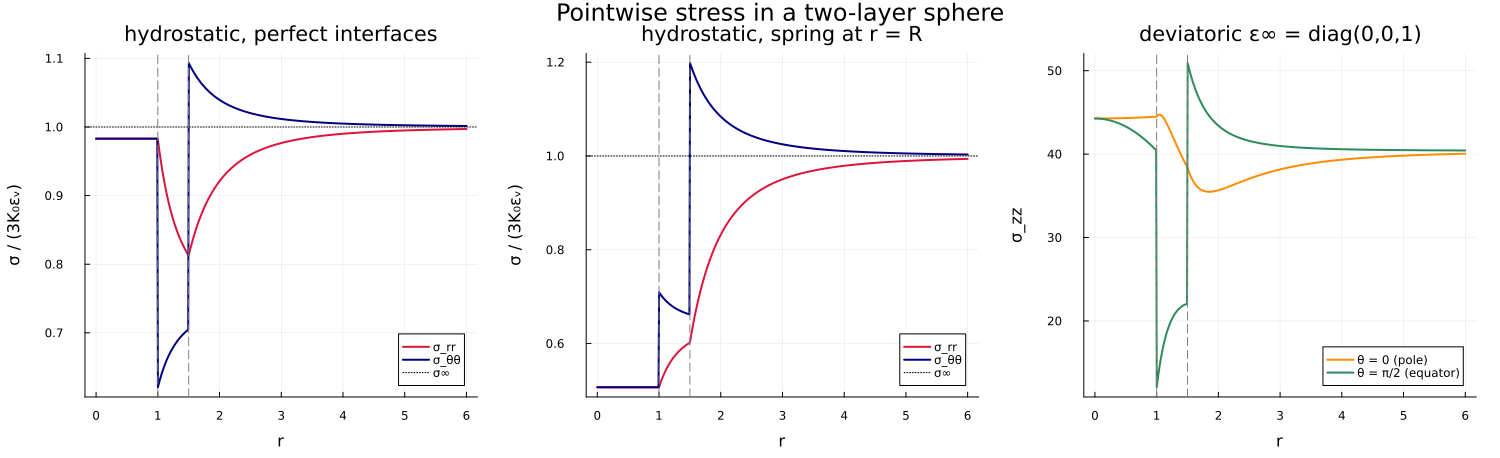
Figure 2 — a meridian map of the von Mises stress
The deviatoric loading breaks the spherical symmetry, so the field is genuinely two-dimensional. A meridian slice
function von_mises(σ)
    s = σ - (tr(σ) / 3) * TensISO{3}(1.0)
    return sqrt(3 / 2 * sum(s[i, j]^2 for i in 1:3, j in 1:3))
end

xs = range(-2.6Rₛ, 2.6Rₛ; length = 220)
zs = range(-2.6Rₛ, 2.6Rₛ; length = 220)
vm = [
    let r = hypot(x, z)
        r < 1.0e-9 ? von_mises(local_stress(sol, [0.0, 0.0, 0.0], ε∞_dev)) :
            von_mises(local_stress(sol, [x, 0.0, z], ε∞_dev))
    end
        for z in zs, x in xs
]

fig2 = heatmap(
    xs, zs, vm;
    aspect_ratio = 1, c = :viridis, xlabel = "x", ylabel = "z",
    title = "von Mises stress, ε∞ = diag(0,0,1)",
    size = (620, 560), right_margin = 6Plots.mm
)
let θ = range(0, 2π; length = 400)
    plot!(fig2, R .* cos.(θ), R .* sin.(θ); lw = 1.5, color = :white, label = "")
    plot!(fig2, Rₛ .* cos.(θ), Rₛ .* sin.(θ); lw = 1.5, color = :white, ls = :dash, label = "")
end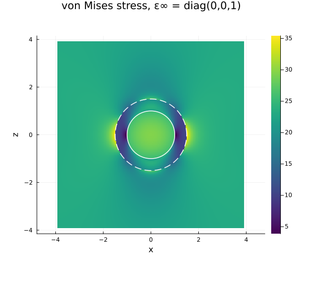
The pointwise field reproduces the layer averages
Averaging shell_localization exposes that identity from the same cached amplitudes, so the two routes cannot drift apart.
println("\nlayer   α_k (pointwise)   α_k (averaged)   β_k (pointwise)   β_k (averaged)")
for k in 1:layer_count(sphere)
    αp, βp = shell_localization(sol, k)
    A = strain_strain_loc(sphere, C₀; layer = k)
    αa, βa = TensND.get_data(A)
    @printf "  %d      %14.10f   %14.10f   %14.10f   %14.10f\n" k αp αa βp βa
end
layer   α_k (pointwise)   α_k (averaged)   β_k (pointwise)   β_k (averaged)
  1        0.4423425706     0.4423425706     0.3273866458     0.3273866458
  2        1.6672912277     1.6672912277     1.6430810955     1.6430810955
This page was generated using Literate.jl.