
Transport properties
Transport properties — diffusivity, permeability, thermal or electrical conductivity — are described by 2nd-order symmetric tensors. They are homogenized with exactly the same machinery as 4th-order elastic properties: only the property key passed to homogenize changes.
Homogenizing a 2nd-order property
A property is stored in each phase under a symbol key — :C for stiffness, :K for conductivity/diffusivity — and selected at homogenization time:
using MeanFieldHomogenization
using TensND
using LinearAlgebra
using Plots
gr()  # headless backend; GKSwstype is set to "100" in make.jl

# Isotropic diffusivities: 2nd-order isotropic tensors.
D_solid = TensISO{3}(0.1)
D_pore = TensISO{3}(1.0)

rve = RVE()
add_phase!(rve, :SOLID, Ellipsoid(1.0, 1.0, 1.0), Dict(:K => D_solid); fraction = :rest)
add_phase!(
    rve, :PORE, Ellipsoid(1.0, 1.0, 0.1), Dict(:K => D_pore);
    fraction = 0.2, symmetrize = IsoSymmetrize()
)

D_eff = homogenize(rve, MoriTanaka(), :K)
tr(Array(D_eff)) / 30.19065028014161733TensISO{3}(k) builds the isotropic 2nd-order tensor
The scheme is a free parameter, exactly as in elasticity:
for scheme in (Dilute(), MoriTanaka(), SelfConsistent())
    D = homogenize(rve, scheme, :K)
    println(rpad(string(nameof(typeof(scheme))), 16), tr(Array(D)) / 3)
end
Dilute 0.18064276801551857
MoriTanaka 0.19065028014161733
SelfConsistent 0.1994431324590776The self-consistent estimate sits above Mori-Tanaka here because the conductive pores percolate in the SC topology, while MT keeps them isolated in a continuous, poorly conductive solid.
Diffusivity of a porous medium
The effective diffusivity of a porous material depends strongly on pore shape, not only on porosity. Flat pores (small aspect ratio
function D_eff_porous(φ, ω; scheme = SelfConsistent())
    r = RVE()
    add_phase!(r, :CEMENT, Ellipsoid(1.0, 1.0, 1.0), Dict(:K => TensISO{3}(0.1)); fraction = :rest)
    add_phase!(
        r, :PORE, Ellipsoid(1.0, 1.0, ω), Dict(:K => TensISO{3}(1.0));
        fraction = φ, symmetrize = IsoSymmetrize()
    )
    return tr(Array(homogenize(r, scheme, :K))) / 3
end

φs = 0.0:0.15:0.6
println("  φ   ", join(["  ω=$ω" for ω in (0.01, 0.1, 1.0, 10.0)]))
for φ in φs
    vals = [D_eff_porous(φ, ω) for ω in (0.01, 0.1, 1.0, 10.0)]
    println(rpad(φ, 6), join([rpad(round(v, digits = 4), 8) for v in vals]))
end
φ ω=0.01 ω=0.1 ω=1.0 ω=10.0
0.0 0.1 0.1 0.1 0.1
0.15 0.186 0.171 0.1457 0.1632
0.3 0.2811 0.2642 0.2261 0.2502
0.45 0.3945 0.3816 0.3503 0.3679
0.6 0.5312 0.5243 0.5084 0.5161The same sweep, plotted as effective diffusivity against porosity for a range of pore aspect ratios
φ_plot = 0.0:0.02:0.6
plt = plot(;
    xlabel = "porosity φ", ylabel = "effective diffusivity D_eff",
    legend = :topleft, framestyle = :box, size = (760, 480),
)
for ω in (0.01, 0.1, 1.0, 10.0)
    plot!(plt, φ_plot, [D_eff_porous(φ, ω) for φ in φ_plot]; label = "ω = $ω", lw = 2)
end
plt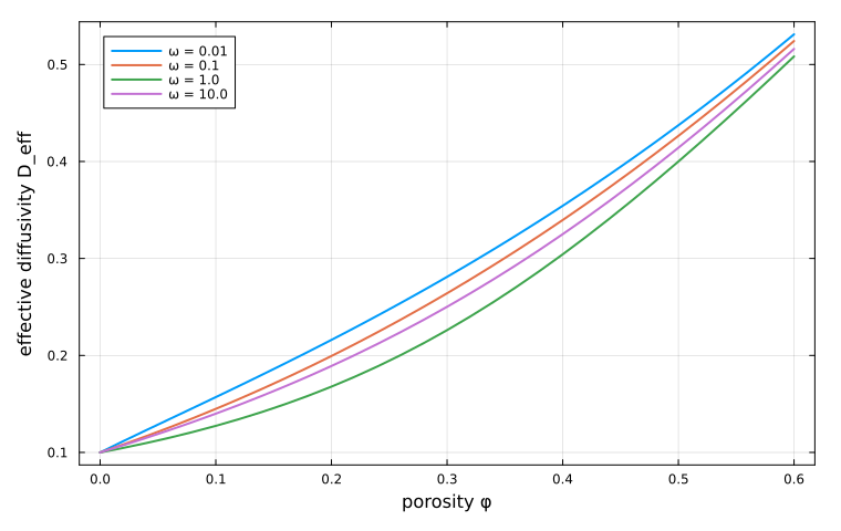
At a given
Two limits are worth checking. At zero porosity every curve must return the solid diffusivity, and at
# Plain bisection — no extra dependency needed.
function bruggeman(φ; Ds = 0.1, Dp = 1.0)
    f(D) = φ * (Dp - D) / (Dp + 2D) + (1 - φ) * (Ds - D) / (Ds + 2D)
    lo, hi = 1.0e-12, 10.0
    for _ in 1:200
        mid = (lo + hi) / 2
        f(lo) * f(mid) <= 0 ? (hi = mid) : (lo = mid)
    end
    return (lo + hi) / 2
end

for φ in (0.2, 0.4, 0.6)
    sc = D_eff_porous(φ, 1.0)
    br = bruggeman(φ)
    println("φ = ", φ, "   SC = ", round(sc, digits = 8),
        "   Bruggeman = ", round(br, digits = 8),
        "   |Δ| = ", round(abs(sc - br), sigdigits = 3))
end
φ = 0.2 SC = 0.16786262 Bruggeman = 0.16786262 |Δ| = 2.27e-10
φ = 0.4 SC = 0.30430749 Bruggeman = 0.30430749 |Δ| = 3.25e-10
φ = 0.6 SC = 0.50835623 Bruggeman = 0.50835623 |Δ| = 2.3e-10The two agree to
Anisotropy induced by oriented pores
If the pores are not re-oriented isotropically, the effective diffusivity inherits their symmetry. Dropping symmetrize = IsoSymmetrize() leaves all pores aligned on
r = RVE()
add_phase!(r, :CEMENT, Ellipsoid(1.0, 1.0, 1.0), Dict(:K => TensISO{3}(0.1)); fraction = :rest)
add_phase!(
    r, :PORE, Ellipsoid(1.0, 1.0, 0.05), Dict(:K => TensISO{3}(1.0));
    fraction = 0.15
)

D_aniso = Array(homogenize(r, MoriTanaka(), :K))
(D_11 = D_aniso[1, 1], D_33 = D_aniso[3, 3])
(D_11 = 0.20527498300671998, D_33 = 0.11669699311419938)The oblate pores lie in the
Sweeping the porosity makes the induced anisotropy explicit — the in-plane and through-thickness diagonal components fan apart as
function D_aniso_components(φ; ω = 0.05)
    r = RVE()
    add_phase!(r, :CEMENT, Ellipsoid(1.0, 1.0, 1.0), Dict(:K => TensISO{3}(0.1)); fraction = :rest)
    add_phase!(
        r, :PORE, Ellipsoid(1.0, 1.0, ω), Dict(:K => TensISO{3}(1.0));
        fraction = φ
    )
    D = Array(homogenize(r, MoriTanaka(), :K))
    return D[1, 1], D[3, 3]
end

φ_plot = 0.0:0.01:0.3
D11 = [D_aniso_components(φ)[1] for φ in φ_plot]
D33 = [D_aniso_components(φ)[2] for φ in φ_plot]
plt2 = plot(;
    xlabel = "porosity φ", ylabel = "effective diffusivity",
    legend = :topleft, framestyle = :box, size = (760, 480),
)
plot!(plt2, φ_plot, D11; label = "D₁₁ (in-plane)", lw = 2)
plot!(plt2, φ_plot, D33; label = "D₃₃ (through-thickness)", lw = 2, ls = :dash)
plt2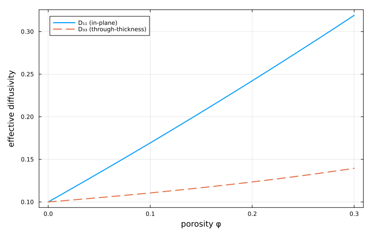
Effect of the Interfacial Transition Zone (ITZ)
In mortar, the Interfacial Transition Zone is a thin shell (~50 µm) of higher-porosity — hence higher-diffusivity — cement paste around each aggregate. The reduction in diffusivity caused by the impermeable aggregates can be offset, or even reversed, by this more permeable surrounding shell.
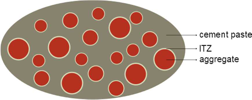
The aggregate + ITZ is a two-layer LayeredSphere — an impermeable core (
const Ragg, eITZ = 5.0e3, 50.0    # µm

function D_itz(f, d_itz)
    f_inc = f * (1 + eITZ / Ragg)^3
    r = RVE()
    add_phase!(r, :CEMENT, Ellipsoid(1.0), Dict(:K => TensISO{3}(1.0)); fraction = :rest)
    agg = LayeredSphere((Ragg, Ragg + eITZ), (TensISO{3}(0.0), TensISO{3}(d_itz)))
    add_phase!(r, :AGG, agg, Dict(:K => TensISO{3}(1.0)); fraction = f_inc)
    return tr(Array(homogenize(r, MoriTanaka(), :K))) / 3
end

# spot values reproduce the Echoes reference exactly
[round(D_itz(0.2, d), digits = 4) for d in (0.001, 50.0, 100.0)]
3-element Vector{Float64}:
0.7198
0.9979
1.1604Sweeping the aggregate fraction for a range of ITZ-to-paste diffusivity ratios
fs = range(0.001, 0.85; length = 40)
plt3 = plot(; xlabel = "aggregate fraction f", ylabel = "D_eff / D_cp",
    legend = :topright, framestyle = :box, ylims = (0, 2), size = (760, 480))
for d in (100.0, 60.0, 50.0, 40.0, 20.0, 0.001)
    lbl = d ≥ 1 ? "D_itz/D_cp = $(Int(d))" : "D_itz/D_cp = 0"
    plot!(plt3, fs, [D_itz(f, d) for f in fs]; lw = 2, label = lbl)
end
plot!(plt3, fs, [(1 - f)^1.5 for f in fs]; c = :black, ls = :dash, label = "(1-f)^{3/2}")
plot!(plt3, fs, [(1 - f) / (1 + 0.5f) for f in fs]; c = :black, ls = :dot, label = "(1-f)/(1+f/2)")
plt3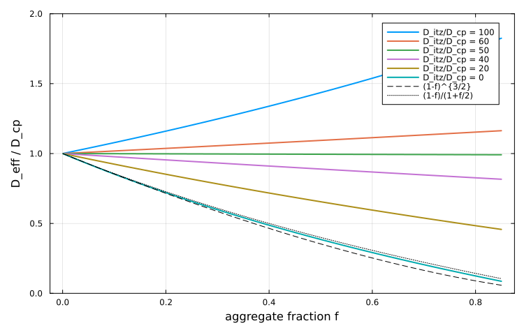
The role of the aggregate + ITZ composite depends strongly on
Zero-thickness interface (DUALDISC)
In the limit DUALDISC model. This is exactly a SurfaceConductiveInterface on a bare aggregate (a one-layer LayeredSphere); it avoids the explicit shell and its volume-fraction correction
function D_dualdisc(f, d_itz)
    α = d_itz * eITZ                                   # transmissivity D_s·e
    agg = LayeredSphere((Ragg,), (TensISO{3}(0.0),);
        interfaces = (SurfaceConductiveInterface(α),))
    r = RVE()
    add_phase!(r, :CEMENT, Ellipsoid(1.0), Dict(:K => TensISO{3}(1.0)); fraction = :rest)
    add_phase!(r, :AGG, agg, Dict(:K => TensISO{3}(1.0)); fraction = f)
    return tr(Array(homogenize(r, MoriTanaka(), :K))) / 3
end

# D_itz/D_cp = 50 makes the surface current exactly offset the impermeable core
[round(D_dualdisc(f, 50.0), digits = 6) for f in (0.1, 0.5, 0.9)]
3-element Vector{Float64}:
1.0
1.0
1.0The surface-conductive interface reproduces the Echoes DUALDISC diffusivity to machine precision, and agrees with the explicit two-layer model up to the small
plt4 = plot(; xlabel = "aggregate fraction f", ylabel = "D_eff / D_cp",
    legend = :topleft, framestyle = :box, ylims = (0, 2), size = (760, 480))
for (d, c) in ((100.0, 1), (50.0, 2), (20.0, 3))
    plot!(plt4, fs, [D_itz(f, d) for f in fs]; lw = 2, c = c,
        label = "layer model — D_itz/D_cp = $(Int(d))")
    plot!(plt4, fs, [D_dualdisc(f, d) for f in fs]; lw = 2, c = c, ls = :dash,
        label = "DUALDISC — D_itz/D_cp = $(Int(d))")
end
plt4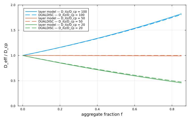
At
Cross-property coupling
Because a single RVE carries several property keys at once, the same microstructure can be homogenized for stiffness and for transport without being rebuilt — which is the basis of cross-property correlations [58]:
r2 = RVE()
add_phase!(r2, :SOLID, Ellipsoid(1.0, 1.0, 1.0), Dict(:C => TensISO{3}(30.0, 12.0), :K => TensISO{3}(0.1)); fraction = :rest)
add_phase!(
    r2, :PORE, Ellipsoid(1.0, 1.0, 0.1),
    Dict(:C => TensISO{3}(1.0e-9, 1.0e-9), :K => TensISO{3}(1.0));
    fraction = 0.15, symmetrize = IsoSymmetrize()
)

C_eff = homogenize(r2, MoriTanaka(), :C)
D_eff2 = homogenize(r2, MoriTanaka(), :K)
(bulk = k_mu(C_eff)[1], diffusivity = tr(Array(D_eff2)) / 3)
(bulk = 4.07913658548325, diffusivity = 0.16594191441863304)