Layered spheroid — confocal harmonic series

LayeredSpheroid is an -layer confocal spheroidal composite inclusion — a core plus concentric confocal shells — embedded in an infinite isotropic matrix, in conduction (thermal, electric, Darcy). It follows [36], which extends the layered-sphere recurrence of [32] to spheroids.

On a sphere an imperfect interface acts on each harmonic degree independently; on a spheroid it couples them. The sphere's   transfer per mode therefore becomes a truncated series with a   transfer matrix per interface.

The elastic problem is on its own page

The axisymmetric elastic case is solved in The elastic confocal spheroid, on the same chart and reusing the same Legendre machinery. It was never barred by the method being tied to the scalar Laplace equation — Barthélémy & Bignonnet say the opposite, that they imported the transfer-matrix formalism from elasticity [36], following Hervé & Zaoui [32] and Hervé & Luanco [34].

What genuinely does not carry over is geometric, and it changes the shape of the answer. Concentric spheres are homothetic, so one harmonic degree never talks to another; confocal spheroids are not, and the metric    leaves factors behind once the denominators are cleared, shifting    . In conduction that coupling appears only at an imperfect interface — which is why the blocks below are diagonal in the perfect case. In elasticity it appears at every interface, perfect ones included, so there is no per-interface transfer matrix to chain at all: the elastic solver assembles one global system instead.

Confocal spheroidal coordinates

Prolate spheroidal coordinates about the revolution axis , with half focal distance  :

with    and  . Surfaces of constant are confocal spheroids — they share the same focal ring, which is what makes the layer geometry consistent — with axial and transverse semi-axes

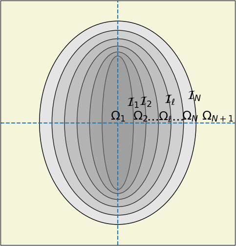
Confocality is a real constraint, and it has a visible consequence: since    is the same for every layer, the inner shells are more elongated than the outer ones. A confocal stack cannot be a set of homothetic shells, and asking for one raises an error at construction. The interactive view in The inclusion zoo shows the effect on a three-layer prolate stack.

Oblate spheroids ( ) follow by the formal substitution    ,    with real, giving    and  . Every prolate formula then carries over unchanged, evaluated in complex arithmetic.

LayeredSpheroid exploits this directly: the confocal parameter is stored as T for a prolate spheroid and Complex{T} for an oblate one, and every downstream routine — Legendre recurrences, coupling integrals, transfer matrices — is written generically over Q <: Number. No branch is ever taken on prolate versus oblate.

The chart, checked rather than quoted

Everything above is Appendix A of [36]. Rather than transcribe it, the block below rebuilds it: TensND ships the prolate spheroidal chart as a symbolic coordinate system, so the metric, the frame and the harmonicity of the series are derived at documentation-build time from the position map alone.

using TensND, SymPy
Spheroidal = coorsys_spheroidal()
ϕ, p, q = getcoords(Spheroidal)
c = symbols("c", positive = true)
getOM(Spheroidal)            # the position map (A.1)

The Lamé coefficients (χ_ϕ, χ_p, χ_q) come out of the chart, not out of the paper:

Lame(Spheroidal)

(c*sqrt(1 - p^2)*sqrt(q^2 - 1), c*sqrt(-p^2 + q^2)/sqrt(1 - p^2), c*sqrt(-p^2 + q^2)/sqrt(q^2 - 1))

and they are (A.6). The check compares the squares — SymPy will not recombine with unless it is told the signs, so the difference of the radicals themselves does not reduce to zero even though they are equal on the domain:

χ = Lame(Spheroidal)
χ_ref = (
    c * sqrt(1 - p^2) * sqrt(q^2 - 1),
    c * sqrt((q^2 - p^2) / (1 - p^2)),
    c * sqrt((q^2 - p^2) / (q^2 - 1)),
)
[simplify(χ[i]^2 - χ_ref[i]^2) for i in 1:3]

The volume element (A.7), dΩ = χ_ϕ χ_p χ_q dϕ dp dq = c³ (q² − p²) dϕ dp dq, follows immediately and does reduce:

simplify(prod(χ) - c^3 * (q^2 - p^2))

and the orthonormal frame (e_ϕ, e_p, e_q) of (A.6) is the chart's own:

normalized_basis(Spheroidal)

Why the series is a series of harmonics

The whole construction rests on one fact: the products    are harmonic. That is what makes a truncated sum of them an admissible temperature field, and it is checked here directly, by applying the chart's Laplacian:

Δ = [
    (n, m, simplify(LAPLACE(
        sympy.assoc_legendre(n, m, p) * sympy.assoc_legendre(n, m, q) * cos(m * ϕ),
        Spheroidal,
    )))
    for (n, m) in ((1, 0), (2, 0), (3, 0), (1, 1), (2, 1), (3, 1), (2, 2), (3, 2))
]

8-element Vector{Tuple{Int64, Int64, SymPyCore.Sym{PyCall.PyObject}}}:
 (1, 0, 0)
 (2, 0, 0)
 (3, 0, 0)
 (1, 1, 0)
 (2, 1, 0)
 (3, 1, 0)
 (2, 2, 0)
 (3, 2, 0)

Orders 0 and 1 are what conduction uses — order 2 is for later

A remote gradient excites only   (axial) and   (transverse), which is why legendre.jl implements exactly those two.   is verified above because the elastic counterpart will need it: a remote transverse shear carries a dependence, and Papkovich–Neuber expands each of its potentials in the very same spheroidal harmonics ([37]). Adding order 2 to legendre.jl is then three seed tables — the stability machinery below is order-generic and comes for free. See the roadmap's checklist.

Boundary value problem

confocal layers of isotropic conductivity , separated by interfaces at   for  , are embedded in a matrix of conductivity occupying  , under a remote uniform gradient . The temperature in layer expands on spheroidal harmonics,

where and are the associated Legendre functions of the first and second kind. By symmetry the problem splits into two independent ones, solved by identical machinery:

problem	remote gradient	order	degrees
axial			odd only
transverse			odd only

An arbitrary remote gradient follows by rotation, the geometry being axisymmetric.

Interface conditions and the coupling matrices

Three interface types are available. Writing   for the jump across the interface and for the normal flux:

type	condition	MeanFieldHomogenization	effect on degrees
perfect	,	PerfectInterface	diagonal
LC (low-conducting)	, flux continuous	KapitzaInterface(ρ)	couples all degrees
HC (highly-conducting)	, temperature continuous	SurfaceConductiveInterface(β)	couples all degrees

The LC model is the Kapitza thermal contact resistance [38], [39]; the HC model is a highly conducting surface layer [40]. Both are the imperfect-interface models used by [41] and [36].

Sign convention

is a genuine thermal resistance and a genuine surface conductance. This is not the inverse convention carried by some raw echoes interf_prop values for the low-conducting case.

The coupling arises because a non-spherical interface mixes harmonic degrees. Four matrices carry it, defined as integrals over the interface [36]:

and similarly , for the transverse HC case. The LC interface couples through (axial) or (transverse); the HC interface through (axial) or    (transverse). They are assembled by coupling_matrices.

Transfer matrices

Truncating at terms — odd degrees   — the interface condition becomes a linear map between the coefficient vectors   of consecutive layers,  , with

where   is diagonal for each of  , and is the interface perturbation: full   blocks built from the coupling matrices above, perturbing the temperature half of for an LC interface and the flux half for an HC one. A perfect interface has  , and only then is diagonal.

Accumulating  , imposing regularity at the core ( ) and the unit remote field (  , axial, transverse) determines every layer's coefficients. This is what spheroid_state_sequence computes, and what local_temperature, local_gradient and local_flux reconstruct pointwise from.

Volume-averaged concentration tensors

For homogenization only two order-2 tensors are needed. They are defined by the volume averages over the whole particle of the gradient and of the flux, under a remote gradient :

is the concentration tensor — how much of the remote gradient the particle actually sees — and the corresponding flux average. Note which flux: the averaged quantity is     , the stress analog of the package (see Elasticity and transport: one set of formulas), so is the exact twin of the elastic with no sign to remember. Both are transversely isotropic, diagonal in the spheroid's own frame, and returned as TensND.TensTI{2,3}.

Remarkably, they depend on the whole layered structure only through the single ratio   of the leading coefficients at the outer boundary , together with four shape functions [36]:

The coincidence   is genuine, not a typo: both equal . Writing for the axial and for the transverse component, and , for the corresponding coefficient ratios,

These are gradient_gradient_loc and flux_gradient_loc.

Like LayeredSphere, a layered spheroid has no Hill tensor — it is not a homogeneous ellipsoid, so does not exist for it. It plugs into the mean-field schemes through and directly, and satisfies the same invariant as the sphere for the size-independent contribution,    .

Equivalent particle

[36] (§4) define the equivalent particle: the homogeneous, perfectly bonded spheroid of the same shape that homogenizes identically. Its conductivity is

with and as defined just above. Unlike a homogeneous perfect-interface spheroid — whose response depends on shape only — is size-dependent, because an imperfect interface introduces a length scale ( and are not dimensionless). Demonstrated in scripts/34_spheroid_equivalent_conductivity.jl.

When every interface is perfect, only degree 1 survives, the coupling matrices drop out, and reduces to the closed-form nested recursion of the paper's §3 — built from the classical conduction depolarization factors already available through tens_IA and hill_tensor for a single spheroid. That closed form is used as an exact oracle in test/LayeredSpheroids/test_conductivity.jl.

Numerical precision: quadrature, not the monomial series

The reference implementation of [36] computes , , , by expanding the products into monomials, with coefficients built by the recursions of the paper's appendix, and summing against

(closed form via ). This is numerically ill-conditioned: the monomial coefficients of a degree- Legendre polynomial grow like , while  . The summation    must therefore cancel terms of size down to a result of size . The paper's own rule of thumb — a working precision of about    decimal digits — is exactly this cancellation bound, and is why the reference implementation needs mpmath arbitrary precision once  .

MeanFieldHomogenization integrates the definitions above directly by Gauss quadrature (QuadGK), evaluating , and their derivatives through the stable three-term recurrence, never through the monomial expansion:

coupling_matrices(q, Nseries; method = :quadrature)   # default
coupling_matrices(q, Nseries; method = :series)       # BigFloat validation oracle

The integrand is smooth and bounded on   for a prolate , and complex-analytic with no real singularity for an oblate  : Float64 quadrature reaches machine precision for any . The BigFloat port of the monomial series is kept as an independent oracle (test/LayeredSpheroids/test_coupling.jl, scripts/33_spheroid_series_convergence.jl).

Integration with the schemes

LayeredSpheroid is wired into the schemes exactly like LayeredSphere (see Layered sphere and src/LayeredSpheres/scheme_integration.jl for the elastic and conduction analogues): it declares is_homogeneous_inclusion = false and overrides gradient_gradient_loc, flux_gradient_loc and conductivity_contribution. Every dilute, Mori–Tanaka, self-consistent, Maxwell and differential kernel then routes through the confocal transfer-matrix solution with no change to src/Schemes/.