The equivalent inclusion method, against a published table

The variational form of the equivalent inclusion method ([65]) is a Galerkin discretization of the weak Lippmann-Schwinger equation. At order p = 0 the polarization is constant over each inclusion and the unknowns solve

being the Hill tensor of the statistical volume element itself — the term that implements their mixed boundary conditions and removes any need for periodization. The package shares the sign convention of [3], so this is transcribed with nothing flipped: the self term is    and every block carries a plus.

Because the method minimizes a Hashin-Shtrikman functional over a finite-dimensional space, the estimate is a rigorous bound whenever the matrix is stiffer (upper) or softer (lower) than every inhomogeneity.

This page reproduces the p = 0 row of their Table 1: plane strain,   circular pores of radius in a circular SVE of radius  , porosity  , matrix  . The paper reports    averaged over 1000 realizations, against a finite-element reference of   and a Hashin-Shtrikman upper bound of  .

Theory: the equivalent inclusion method.

using MeanFieldHomogenization
using TensND
using Random
using Printf
using Plots
gr()

default(; left_margin = 5Plots.mm, bottom_margin = 5Plots.mm)

Random.seed!(20260810)

Random.TaskLocalRNG()

Setting

Plane strain with μ₀ = 1 and ν₀ = 0.3. In two dimensions TensISO{2}(α, β) is     with    the plane-strain area modulus. The pores are given a vanishing stiffness rather than exactly zero, so that the contrast   stays invertible.

μ₀, ν₀ = 1.0, 0.3
κ₂ = μ₀ / (1 - 2ν₀)
C_m = TensISO{2}(2κ₂, 2μ₀)
C_void = TensISO{2}(2κ₂ * 1.0e-9, 2μ₀ * 1.0e-9)

a, N, R = 1.0, 160, 20.0
@printf "porosity φ = N a² / R² = %.3f\n" N * a^2 / R^2

porosity φ = N a² / R² = 0.400

One realization

The microstructure is generated by the hard-particle Metropolis algorithm of the paper's §5: the disks start on a regular grid inside the SVE and are then shuffled, the move amplitude being retuned every 50 sweeps to hold the acceptance ratio near 0.3.

rng = Random.MersenneTwister(20260810)
asm = random_assembly(
    N, Dict(:C => C_m), Dict(:C => C_void);
    radius = a, dim = 2, rng = rng, cycles = 4000,
    boundary = MixedBC(Ellipsoid(R, R))
)
println(asm)
println("bound type: ", eim_bound_type(asm))

C = homogenize(asm, EquivalentInclusion(), :C)
@printf "μ_app / μ₀ = %.4f   (single realization)\n" get_array(C)[1, 2, 1, 2] / μ₀

ParticleAssembly(160 particles, MixedBC, f = 0.4)
bound type: upper
μ_app / μ₀ = 0.3019   (single realization)

Monte-Carlo over realizations

The published value averages 1000 microstructures; a few dozen already put the statistical error well below the gap to the reference.

nreal = 8            ## reduced ensemble, so the documentation build stays cheap
vals = Float64[]
for m in 1:nreal
    asm_m = random_assembly(
        N, Dict(:C => C_m), Dict(:C => C_void);
        radius = a, dim = 2, rng = rng, cycles = 4000,
        boundary = MixedBC(Ellipsoid(R, R))
    )
    push!(vals, get_array(homogenize(asm_m, EquivalentInclusion(), :C))[1, 2, 1, 2] / μ₀)
end

mean_val = sum(vals) / length(vals)
sem = sqrt(sum((v - mean_val)^2 for v in vals) / max(1, length(vals) - 1)) / sqrt(length(vals))
@printf "\nEIM (p = 0), %d realizations : μ_app/μ₀ = %.4f ± %.4f\n" length(vals) mean_val sem
@printf "paper (1000 realizations)     : 0.310\n"
@printf "finite-element reference      : 0.244\n"
@printf "Hashin-Shtrikman upper bound  : 0.349\n"

EIM (p = 0), 8 realizations : μ_app/μ₀ = 0.3087 ± 0.0020
paper (1000 realizations)     : 0.310
finite-element reference      : 0.244
Hashin-Shtrikman upper bound  : 0.349

Reading the result

The estimate sits between the finite-element value it bounds from above and the Hashin-Shtrikman bound it improves on. Both statements are what the variational structure guarantees: taking the polarization constant and equal across all inclusions recovers Hashin-Shtrikman, and letting it vary from one inclusion to the next can only lower an upper bound.

p1 = scatter(
    1:length(vals), vals;
    xlabel = "realization", ylabel = "μ_app / μ₀",
    title = "EIM (p = 0), $(N) circular pores, φ = 0.4",
    label = "EIM", ms = 4, legend = :right
)
hline!(p1, [mean_val]; label = @sprintf("mean = %.4f", mean_val))
hline!(p1, [0.310]; ls = :dash, label = "paper, p = 0")
hline!(p1, [0.349]; ls = :dot, label = "HS upper bound")
hline!(p1, [0.244]; ls = :dashdot, label = "FEM reference")
p1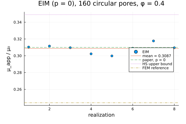

The microstructure

Worth a look: this is the geometry the estimate is computed on — 160 non-overlapping disks inside a circular SVE, not a periodic cell.

θ = range(0, 2π; length = 200)
p2 = plot(
    R .* cos.(θ), R .* sin.(θ);
    aspect_ratio = 1, color = :black, lw = 2, label = "SVE",
    xlabel = "x", ylabel = "y", title = "One realization", legend = false
)
for nm in particle_names(asm)
    c = particle_center(asm, nm)
    plot!(p2, c[1] .+ a .* cos.(θ), c[2] .+ a .* sin.(θ); seriestype = :shape,
        fillalpha = 0.5, lw = 0.4, color = :steelblue, label = "")
end
p2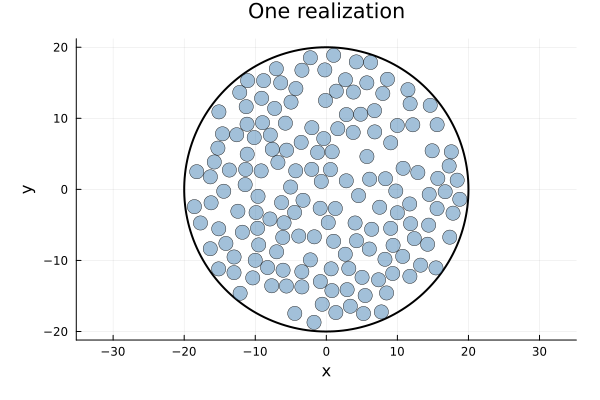

Effect of the porosity

At fixed SVE size, adding pores drives the apparent modulus down; the EIM estimate stays an upper bound throughout because the matrix is stiffer than every inhomogeneity.

φs = [0.1, 0.2, 0.3, 0.4]
μs = Float64[]
for φ in φs
    Nφ = round(Int, φ * R^2 / a^2)
    asm_φ = random_assembly(
        Nφ, Dict(:C => C_m), Dict(:C => C_void);
        radius = a, dim = 2, rng = rng, cycles = 4000,
        boundary = MixedBC(Ellipsoid(R, R))
    )
    push!(μs, get_array(homogenize(asm_φ, EquivalentInclusion(), :C))[1, 2, 1, 2] / μ₀)
    @printf "φ = %.2f  (N = %3d)  μ_app/μ₀ = %.4f\n" φ Nφ μs[end]
end

p3 = plot(
    φs, μs; marker = :circle, ms = 4,
    xlabel = "porosity φ", ylabel = "μ_app / μ₀",
    title = "EIM (p = 0) vs porosity", label = "EIM", legend = :topright
)
scatter!(p3, [0.4], [0.310]; ms = 6, marker = :star5, label = "paper, φ = 0.4")
p3

p_full = plot(p1, p2, p3; layout = (1, 3), left_margin = 8Plots.mm, bottom_margin = 8Plots.mm,
    size = (1500, 520), titlefontsize = 9)
p_full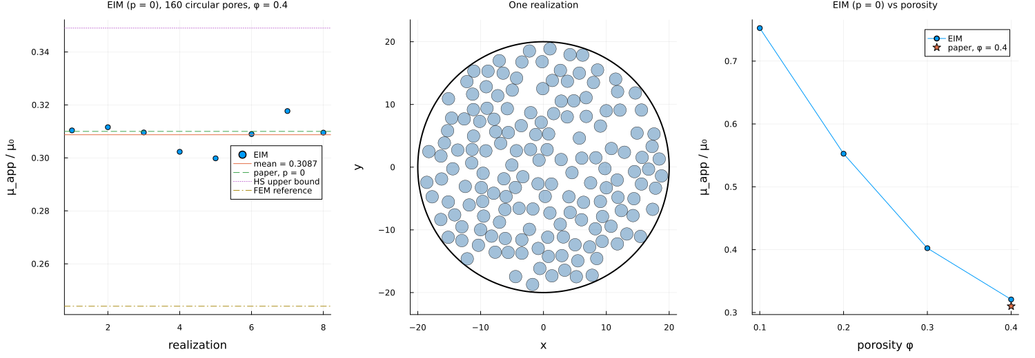

---

This page was generated using Literate.jl.