Quasi-brittle strength of cement paste and mortar

This chapter implements the multi-scale strength-upscaling model of [72] — and mirrors the corresponding chapter of the Echoes book [73]. It predicts the macroscopic uniaxial compressive strength of a mortar from the strength of a single hydrate phase, by upscaling through three nested homogenization scales.

Scale	RVE	Phases	Scheme
1	Hydrate foam (HF)	oriented hydrate needles + water + air	Self-Consistent
2	Cement paste (CP)	HF matrix + clinker grains	Mori-Tanaka
3	Mortar (MO)	CP matrix + sand grains	Mori-Tanaka

The criterion needs , propagated through all three scales. Echoes assembles it by an explicit chain rule over the five transversely-isotropic parameters of every intermediate tensor; here it is a single ForwardDiff pass through the whole nested chain — make the   family's shear modulus a Dual, read the partial of the final C_mo. Both routes agree to the tolerances of Cross-validation.

The code below is the model of scripts/common/quasibrittle_strength.jl, reproduced inline.

Constants and volume fractions

Densities (relative to water) and phase moduli are those of [72]. Powers' hydration model gives the volume fractions of clinker, water, hydrates and air as functions of and the hydration degree ( ); the sand fraction follows from the sand-to-cement ratio .

using MeanFieldHomogenization
using TensND
using ForwardDiff
using LinearAlgebra
using Plots
gr()  # headless backend; GKSwstype is set to "100" in make.jl

const d_clin, d_hyd, d_san = 3.15, 2.073, 2.648
const K_clin, μ_clin = 116.7, 53.8
const K_hyd_ref, μ_hyd_ref = 18.7, 11.8
const K_san, μ_san = 37.8, 44.3

# Water/air are regularized to a tiny positive stiffness: it selects the
# percolating SC branch and keeps the iteration smooth (deliberate deviation
# from the exact zero — the source of the ~2% f_c gap with Echoes).
const TINY = 1.0e-3
const NTHETA = 20
const ω_aspect = 1.0e4

f_clin(wc, α) = (1 - α) / (1 + d_clin * wc)
f_w(wc, α) = d_clin * (wc - 0.42α) / (1 + d_clin * wc)
f_hyd(wc, α) = 1.42 * d_clin / d_hyd * α / (1 + d_clin * wc)
fh_san(wc, sc) = sc / d_san / (1 / d_clin + wc + sc / d_san)
αmax(wc) = min(1.0, wc / 0.42)

Scale 1 — hydrate foam (multi-bin self-consistent)

The hydrate crystals are near-perfect needles (prolate spheroids,  ) with a random orientation distribution. The distribution is discretized into NTHETA polar bins (polar_orientation_bins); each bin is one Spheroid family tilted by its polar angle and carrying a TISymmetrize — the exact azimuthal average about the global axis , preserving the non-major-symmetric content of the concentration tensors. The foam (needles + water + air) is homogenized self-consistently. The shear modulus of the first family ( ) is kept as a separate argument μ_b0 so it can later be seeded with a ForwardDiff.Dual.

function build_hf(wc, α_p, μ_b0; N = NTHETA, ω = ω_aspect)
    fclin, fw, fhyd = f_clin(wc, α_p), f_w(wc, α_p), f_hyd(wc, α_p)
    fair = max(0.0, 1 - fclin - fw - fhyd)
    fthyd, ftw, ftair = fhyd / (1 - fclin), fw / (1 - fclin), fair / (1 - fclin)

    T = typeof(μ_b0)
    ez = (0.0, 0.0, 1.0)
    rve = RVE(; T = T)
    # Zero-volume matrix = SC seed only (Σ inclusion fractions = 1).
    add_phase!(rve, :CP, Ellipsoid(1.0), Dict(:C => TensISO{3}(convert(T, 3K_hyd_ref), convert(T, 2μ_hyd_ref))); fraction = :rest, symmetrize = :iso)
    for (i, bin) in enumerate(polar_orientation_bins(N))
        μ_h = i == 1 ? μ_b0 : convert(T, μ_hyd_ref)
        add_phase!(
            rve, Symbol(:HYD, i),
            Spheroid(ω; euler_angles = (bin.θ, 0.0, 0.0)),
            Dict(:C => TensISO{3}(convert(T, 3K_hyd_ref), 2μ_h));
            fraction = fthyd * bin.weight, symmetrize = TISymmetrize(ez)
        )
    end
    C_tiny = TensISO{3}(convert(T, 3TINY), convert(T, 2TINY))
    add_phase!(rve, :W, Ellipsoid(1.0), Dict(:C => C_tiny); fraction = ftw, symmetrize = :iso)
    add_phase!(rve, :AIR, Ellipsoid(1.0), Dict(:C => C_tiny); fraction = ftair, symmetrize = :iso)
    return homogenize(
        rve, SelfConsistent(; abstol = 1.0e-8, maxiters = 1000, damping = 0.5),
        :C; select_best = true
    )
end

Scales 2 and 3 — cement paste and mortar (Mori-Tanaka)

The converged foam is a TensTI{4}; best_fit_ti extracts its physical 5-parameter TI stiffness (Echoes does the same with tensor(C_hf.array, TI)) before the two Mori-Tanaka stages: clinker grains in the foam matrix (CP), then sand grains in the paste matrix (MO).

function build_cp(wc, α_p, C_hf)
    T = eltype(C_hf)
    rve = RVE(; T = T)
    add_phase!(rve, :CP, Ellipsoid(1.0), Dict(:C => C_hf); fraction = :rest)
    add_phase!(
        rve, :CLIN, Ellipsoid(1.0),
        Dict(:C => TensISO{3}(convert(T, 3K_clin), convert(T, 2μ_clin)));
        fraction = f_clin(wc, α_p)
    )
    return homogenize(rve, MoriTanaka(), :C)
end

function build_mo(wc, sc, C_cp)
    T = eltype(C_cp)
    rve = RVE(; T = T)
    add_phase!(rve, :CP, Ellipsoid(1.0), Dict(:C => C_cp); fraction = :rest)
    add_phase!(
        rve, :SAN, Ellipsoid(1.0),
        Dict(:C => TensISO{3}(convert(T, 3K_san), convert(T, 2μ_san)));
        fraction = fh_san(wc, sc)
    )
    return homogenize(rve, MoriTanaka(), :C)
end

# Full chain: scalar μ_b0 in, C_mo array out.
function multiscale_C_mo(wc, α_p, sc, μ_b0; N = NTHETA, ω = ω_aspect)
    C_hf = best_fit_ti(build_hf(wc, α_p, μ_b0; N = N, ω = ω), (0.0, 0.0, 1.0))
    C_cp = build_cp(wc, α_p, C_hf)
    C_mo = build_mo(wc, sc, C_cp)
    return get_array(C_mo)
end

Strength criterion and the autodiff sensitivity

The compliance pull-back     gives the axial term , and [72]'s criterion reads

where is the mortar volume fraction of the perturbed ( ) hydrate family. The sensitivity is obtained by seeding with a Dual and reading the partial of the final array — one pass through the whole three-scale chain.

extract_kμ(arr) = k_mu(TensND.proj_tens(Val(:ISO), arr)[1])

function quasibrittle_strength(arr_C_mo, arr_dC, μh, f_θ)
    # `arr_C_mo` (value) and `arr_dC` (∂/∂μ) are 3×3×3×3 arrays; wrap them as
    # `Tens` and use intrinsic TensND algebra — the effective compliance is the
    # full inverse and the pull-back is one double contraction, no index loops.
    S = inv(Tens(arr_C_mo))
    M = S ⊡ Tens(arr_dC) ⊡ S
    return 1 / sqrt(abs(M[3, 3, 3, 3]) * 2μh^2 / f_θ)
end

function compute_point(wc, α_p; sc = 0.0, N = NTHETA, ω = ω_aspect)
    TagT = typeof(ForwardDiff.Tag(multiscale_C_mo, Float64))
    μ_dual = ForwardDiff.Dual{TagT}(float(μ_hyd_ref), 1.0)
    arr = multiscale_C_mo(wc, α_p, sc, μ_dual; N = N, ω = ω)
    arr_C = ForwardDiff.value.(arr)
    arr_dC = ForwardDiff.partials.(arr, 1)

    K_mo, μ_mo = extract_kμ(arr_C)
    E_mo, _ = E_nu(iso_stiffness(K_mo, μ_mo))
    f_θ = f_hyd(wc, α_p) * (1 - fh_san(wc, sc)) * polar_orientation_bins(N)[1].weight
    # criterion uses the iso parameter 2μ: d/d(2μ) = (1/2) d/dμ
    fc = quasibrittle_strength(arr_C, arr_dC ./ 2, μ_hyd_ref, f_θ)
    return (; K_mo, μ_mo, E_mo, fc)
end

r = compute_point(0.5, αmax(0.5) * (1 - 1e-12))
(k = round(r.K_mo, digits = 3), μ = round(r.μ_mo, digits = 3),
    E = round(r.E_mo, digits = 2), fc = round(r.fc, digits = 4))

(k = 12.27, μ = 8.055, E = 19.83, fc = 1.1024)

The rest of the chapter uses this single-pass sensitivity throughout. The following section is a pedagogical aside — it opens the black box to show what that one autodiff pass computes internally, and how it relates to the explicit chain rule of the original Echoes implementation. It is not needed to run the model.

Under the hood: the multi-scale chain rule made explicit

Two routes to the same derivative

The sensitivity spans three homogenization scales. There are two ways to obtain it, and they are mathematically identical:

• Direct (used above) — seed as a ForwardDiff.Dual and let it propagate through the entire nested chain build_hf → build_cp → build_mo in one evaluation. The chain rule happens automatically inside the dual-number arithmetic; you write no derivatives by hand.

• Explicit chain rule (this section, the Echoes approach) — differentiate each scale separately with respect to its input tensor, then multiply the per-scale Jacobians. Echoes assembles exactly this product with one homogenize_derivative call per transversely-isotropic (TI) parameter, per scale.

The explicit route is more work, but it makes the structure visible — and it reveals a key fact: because every intermediate stiffness is transversely isotropic (aligned needles in an isotropic matrix, then spherical clinker and sand), only five numbers — the TI parameters — flow between scales.

The bridge between the two views is the TI parameterization: extract the five parameters of a tensor with best_fit_ti — one of the symmetry projections re-exported from TensND — and rebuild a TensTI from five numbers.

const ez = (0.0, 0.0, 1.0)
ti5(C) = collect(TensND.get_data(best_fit_ti(C, ez)))     # tensor → 5 TI params
function rebuildTI(p)                                     # 5 params → TensTI
    T = eltype(p)
    return TensTI{4, T, 5}((p[1], p[2], p[3], p[4], p[5]),
        (T(ez[1]), T(ez[2]), T(ez[3])))
end

Now the three per-scale Jacobians, each a small ForwardDiff problem in the 5-parameter space rather than a pass through the whole model:

wc, α, sc = 0.5, αmax(0.5) * (1 - 1e-9), 0.0

# Scale 1 — how the five HF parameters respond to μ_hyd  (5-vector)
p_hf0 = ti5(build_hf(wc, α, μ_hyd_ref))
dHF_dμ = ForwardDiff.derivative(μ -> ti5(build_hf(wc, α, μ)), float(μ_hyd_ref))

# Scale 2 — how the CP parameters respond to the HF parameters  (5×5)
p_cp0 = ti5(build_cp(wc, α, rebuildTI(p_hf0)))
J_cp = ForwardDiff.jacobian(p -> ti5(build_cp(wc, α, rebuildTI(p))), p_hf0)

# Scale 3 — how the full mortar stiffness responds to the CP parameters  (81×5)
J_mo = ForwardDiff.jacobian(p -> vec(get_array(build_mo(wc, sc, rebuildTI(p)))), p_cp0)

(size_dHF_dμ = size(dHF_dμ), size_J_cp = size(J_cp), size_J_mo = size(J_mo))

(size_dHF_dμ = (5,), size_J_cp = (5, 5), size_J_mo = (81, 5))

The chain rule is now literally a product of these Jacobians —     — and it reproduces the single-pass result to machine precision:

dCmo_chain = reshape(J_mo * (J_cp * dHF_dμ), 3, 3, 3, 3)

# same quantity, straight from one Dual pass through the whole chain
TagT = typeof(ForwardDiff.Tag(multiscale_C_mo, Float64))
μ_dual = ForwardDiff.Dual{TagT}(float(μ_hyd_ref), 1.0)
dCmo_direct = ForwardDiff.partials.(multiscale_C_mo(wc, α, sc, μ_dual), 1)

maxdiff = maximum(abs, dCmo_chain .- dCmo_direct)
println("max |chain rule − direct pass| = ", round(maxdiff, sigdigits = 3))

max |chain rule − direct pass| = 2.17e-19

Same numbers, but the chain rule requires knowing the intermediate symmetry, choosing a consistent parameter ordering, and assembling the Jacobian product by hand — three opportunities for error that grow with the number of scales. The ForwardDiff pass differentiates whatever the model actually computes.

Results — strength and stiffness vs hydration degree

For pure cement paste ( ), the effective bulk and shear moduli and the normalized compressive strength all rise monotonically with hydration and fall with — the trend reported by [72].

wc_list = (0.25, 0.35, 0.5, 0.65)

pk = plot(; xlabel = "α", ylabel = "k_mortar (GPa)", legend = :topleft, framestyle = :box)
pμ = plot(; xlabel = "α", ylabel = "μ_mortar (GPa)", legend = false, framestyle = :box)
pfc = plot(; xlabel = "α", ylabel = "f_c / σ_ult", legend = false, framestyle = :box)

for wc in wc_list
    αs = range(0.05, αmax(wc) * (1 - 1e-9); length = 14)
    ks, μs, fcs, ak = Float64[], Float64[], Float64[], Float64[]
    for α in αs
        try
            r = compute_point(wc, α)
            push!(ak, α); push!(ks, r.K_mo); push!(μs, r.μ_mo); push!(fcs, r.fc)
        catch
        end
    end
    plot!(pk, ak, ks; label = "w/c=$wc", lw = 2)
    plot!(pμ, ak, μs; lw = 2)
    plot!(pfc, ak, fcs; lw = 2)
end

plot(pk, pμ, pfc; layout = (1, 3), left_margin = 8Plots.mm, bottom_margin = 8Plots.mm, size = (1200, 430),
    plot_title = "Cement paste (s/c = 0)")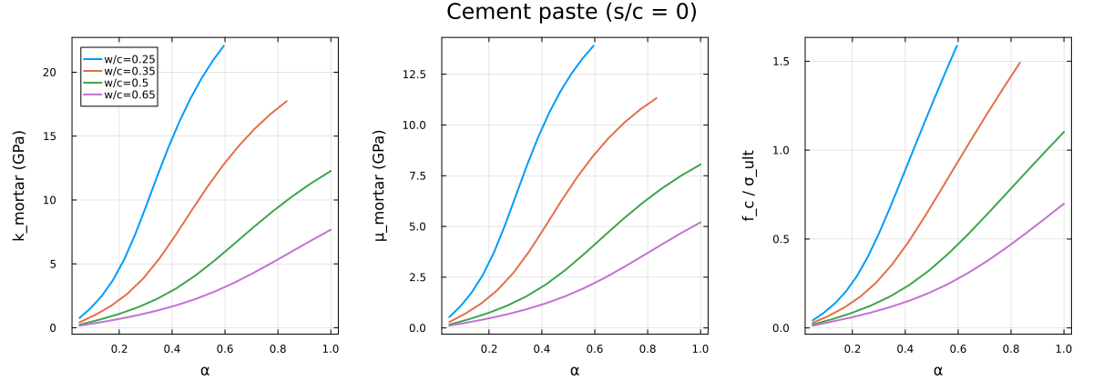

Effect of the sand content

Adding sand (increasing ) dilutes the load-bearing hydrate foam and lowers the normalized strength at full hydration, the effect being sharper at low :

psc = plot(; xlabel = "sand-to-cement ratio s/c", ylabel = "f_c / σ_ult",
    legend = :topright, framestyle = :box, size = (720, 440))
for wc in (0.35, 0.5, 0.65)
    scs = range(0.0, 5.0; length = 12)
    vals, kept = Float64[], Float64[]
    for sc in scs
        try
            fc = compute_point(wc, αmax(wc) * (1 - 1e-9); sc = sc).fc
            fc > 0 && (push!(kept, sc); push!(vals, fc))
        catch
        end
    end
    plot!(psc, kept, vals; label = "w/c=$wc", lw = 2, marker = :circle, ms = 3)
end
psc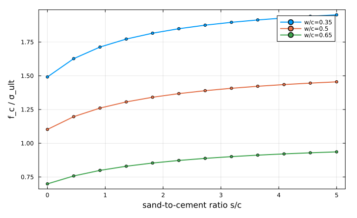

The absolute strength in MPa is recovered by multiplying by , which [72] calibrate to ≈ 70–90 MPa for typical C-S-H.

The same chain, written declaratively

The model above is the explicit multiscale style: one function per scale, each handing its result to the next, and — because the whole chain has to be differentiated at once — a hand-rolled ForwardDiff.Tag seeded into μ_b0 and read back out of the final array.

The declarative style writes the same chain as a single object, a phase property being another cell plus a scheme. Here the last two scales are plain Mori-Tanaka stages with nothing in between, so they port directly:

function cp_mo_declarative(wc, sc, α_p, C_hf)
    T = eltype(C_hf)
    cp = RVE(; T = T)
    add_phase!(cp, :HF, Ellipsoid(1.0), Dict(:C => C_hf); fraction = :rest)
    add_phase!(cp, :CLIN, Ellipsoid(1.0),
        Dict(:C => TensISO{3}(convert(T, 3K_clin), convert(T, 2μ_clin)));
        fraction = f_clin(wc, α_p))

    mo = RVE(; T = T)
    add_phase!(mo, :CP, Ellipsoid(1.0), Dict(:C => Homogenized(cp, MoriTanaka())); fraction = :rest)
    add_phase!(mo, :SAN, Ellipsoid(1.0),
        Dict(:C => TensISO{3}(convert(T, 3K_san), convert(T, 2μ_san)));
        fraction = fh_san(wc, sc))
    return mo
end

let wc = 0.5, sc = 0.0, α_p = αmax(0.5) * (1 - 1e-12)
    C_hf = best_fit_ti(build_hf(wc, α_p, float(μ_hyd_ref)), (0.0, 0.0, 1.0))
    C_explicit = build_mo(wc, sc, build_cp(wc, α_p, C_hf))
    C_declarative = homogenize(cp_mo_declarative(wc, sc, α_p, C_hf), MoriTanaka(), :C)
    maximum(abs, get_array(C_explicit) - get_array(C_declarative))
end

0.0

Identical to the last bit — as it must be: the two styles differ in how the chain is written, not in what it computes.

Why the foam stage keeps its explicit form here

The seam between the hydrate foam and the cement paste is not a plain hand-off: the converged TensTI{4,T,8} is passed through best_fit_ti before the Mori-Tanaka stage, to match what Echoes does. A Homogenized resolves to whatever the inner scheme returns, so a post-processing step of that kind has to happen outside it.

That is the general rule stated in Multiscale models: the declarative style is for chains whose scales hand results straight to one another; a scale that needs a projection, a criterion or a change of variables in between keeps its explicit form. Both styles are first-class, and mixing them — as here, explicit at the foam seam and declarative afterwards — is normal.

What the declarative form would buy

Where a chain is fully declarative, the sensitivity plumbing disappears: the ForwardDiff.Tag seeding above is replaced by a lens naming the parameter, wherever it lives in the chain,

p = nested(:CP, :C, property(:HF, :C, :shear))    # μ of the foam, one scale down
gradient(mo, MoriTanaka(), [p]; indexer = C -> k_mu(C)[2])

and the inner cells are still solved exactly once per evaluation. The three-scale worked example is the multiscale tutorial, which writes one model both ways and checks that the derivatives agree with finite differences.