The finite Eshelby cell with a corrected boundary condition

When a morphology has no closed-form Eshelby solution, its response can be computed on a finite cell — the inclusion inside a ball of matrix of radius — and fed to the schemes through the custom-inclusion contract. The difficulty is that Eshelby's problem is posed on an infinite medium. This page states the first-order correction of [68], which removes the truncation bias, in the general form and in the two declinations the package implements.

The finite-size bias

We want the response of an infinite medium, but we can only mesh a finite ball of radius . The obvious boundary condition is the remote field itself,

but it clamps the perturbation radiated by the crack: the boundary is not allowed to move the way the infinite medium would let it. The apparent opening therefore carries a bias of order , which is why an uncorrected computation needs R/a between 10 and 40 before it can be trusted.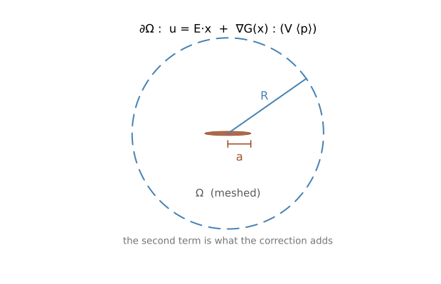

Without the dipole term the boundary carries the remote field alone, and the ball has to be made large enough for the neglected term to fall below the target accuracy. With it, the boundary already knows what the infinite medium would do, and R/a = 5 suffices — the default radius_ratio of the finite-element backends (FE inclusions) — the price being that appears on both sides.

The general fixed point

The exact infinite-medium solution is

whose far field, since    when  , collapses to a single force dipole:

Imposing    on a sphere of radius therefore leaves an bias. Adding the dipole term removes it, at the price of a fixed point, because is itself an output of the problem.

Split by linearity into two boundary-value problems on the truncated cell:

Superposing and demanding that be the polarization it generates,

which is linear in and solves in closed form:

Two declinations are implemented, and they differ only in what carries the polarization:

	solid inclusion	crack	cavity
unknown	on the Kelvin basis		itself
solves	6 + 6, or 2 + 2 per Fourier mode	3 + 3	6 + 6, or 2 + 2 and 1 + 1 per mode
closes on
used by	FEExcenteredSphere, FEAxiLayeredSpheroid	FEEllipticCrack	FESupershapePore, FEAxiSupershapePore

In the axisymmetric case each fixed point lives inside one Fourier mode, since the dipole of a modal polarization radiates in the same mode — so is   for mode 0 and a scalar for modes 1 and 2.

The dipole fields, in closed form

For an isotropic reference medium both Green functions are closed forms, so the boundary data costs nothing. With  ,   and   the polarization moment, the elastic field is dipole_displacement_iso:

Written out for a symmetric moment, the gradient of the Kelvin solution is

and the transport one, with  ,

These are green_gradient_iso and dipole_displacement_iso. They are also why the reference medium must be isotropic: for arbitrary anisotropy would come from the Willis integral, or from the Pan–Chou closed form in the transversely isotropic case, neither of which is implemented.

The pore declination

A cavity is its own polarization source

The general fixed point above needs the polarization of the inclusion, and for a cavity that quantity is not something extra to compute: it is the answer. A cavity carries no stress, so

the very tensor being measured. So the two-stage construction — solve for , solve for , then invert for — collapses. Writing for the response to the remote field alone and for the response to a unit dipole, the loop closes in one inversion:

There is no anywhere in it, which is the point: inv(C₁) is meaningless for a cavity, and this is why FESupershapePore declares itself a heterogeneous inclusion and lets the package's exact identities collapse to     and   .

The two signs, and why they are not inconsistent

carries a minus in both physics, and the transport one looks like it should not. It is structural. Elasticity pairs      with a polarization , while transport pairs    : splitting the flux as    gives   , and it is that belongs with the temperature   .

The failure mode is worth remembering, because it does not look like a sign error. A wrong sign leaves exactly twice the truncation bias instead of none — the correction is applied backwards, so it adds what it should have subtracted. The result still converges under refinement, just to the wrong place, and only a radius sweep exposes it.

What is solved, and on what volume

Zero traction on the cavity wall in elasticity, zero normal flux in transport. Nothing is meshed inside: the cell is a shell of matrix between the shape and the outer sphere. Two consequences the implementation leans on — the stress-side localization is identically zero, so gate B is served by one tensor rather than two; and the normalizing volume is the curved volume of the cavity, fe_cell_curved_volume, not the volume of the flat triangulation that bounds the mesh, which differs from it by a percent at usable refinements.

The diagnostic is  , which is — measured at a log-log slope of against from theory.

Or two dimensions, when the body is a solid of revolution

An octant divides the cost by eight. Separating the azimuth into Fourier modes divides it by orders of magnitude, and for an axisymmetric cavity that is the route FEAxiSupershapePore takes. Each mode is a problem on the meridian half-plane, and the modes do not couple, so a macroscopic loading excites exactly one of them:

loading	mode	what it yields
,	0	a   block
	1	a scalar
	2	a scalar
/	0 / 1	a scalar each

Three from the   block, one from mode 1, one from mode 2: exactly the five constants of a transversely isotropic compliance contribution, with modes 0 and 1 giving the two of the resistivity. The count is not a coincidence to be checked afterwards — it is the same representation theory in both places.

The fixed point lives inside one mode, since the dipole of a modal polarization radiates in the same mode, so is   for mode 0 and a scalar for modes 1 and 2.

And the averaging changes. A cavity has no interior, so is a boundary integral — over the meridian trace of the wall, with the measure  .

There is a tempting way round it. The divergence identity on the matrix,

gives the cavity average from the volume average over the matrix plus an outer term that is analytic, the datum there being imposed. It reuses only machinery that already exists. It is also numerically hopeless: it obtains as the difference of and , whose ratio is . Two digits go at   and more as the cell grows — the opposite of what a larger cell is for. Measured before it was abandoned: the implied cavity volume is 2.9 % wrong at   and 9.2 % at 216, with the localization error tracking it, and convergence of where the direct route gives more.

One consequence of that route is worth keeping even after abandoning it: normalize by the volume the meshed wall actually encloses, not by the closed form. Integrating over one boundary and dividing by another's volume leaves a systematic error of the geometry's own size, and refining removes none of it because it shrinks both together.

The solid declination in two dimensions, and its region count

An N-layer spheroid is the solid declination of the same correction — and are not zero, and both outputs of the fixed point are used, the second being gate B's stress side. So the cavity was the easy case: it degenerates the correction to      with one useful output, where a heterogeneous inclusion carries the pair.

Nothing else changes. The same three modes, the same two families of boundary data, the same single factorization per mode — and the inclusion average runs over N regions instead of two, which is the only place the layer count appears at all. The dipole's moment is that of the outer boundary, the inclusion being seen from outside: on a multilayer, using an inner layer's volume gives an answer that is almost right.

Two exact answers, and why they are exact

Two numbers from this construction are worth reading as statements rather than as measurements.

Transverse isotropy holds to round-off. For an axisymmetric cavity,    and the normal-to-shear block vanishes, both to and at any refinement, because the modes are decoded straight onto the Kelvin basis. It is therefore a free check that the three modes, the azimuthal projections, the boundary integral and the reassembly are simultaneously right — which is more than any one of them could establish alone.

Conduction on a sphere is exact, and does not improve with refinement. The exterior perturbation of a spherical cavity is a pure dipole, so the corrected boundary condition has no higher multipole left to truncate: the answer sits at   of and stays there. In elasticity, where higher multipoles do exist, what remains is truncation and the radius sweep says so — the uncorrected answer falls as , the signature, and the corrected one as .

One eighth of the cell

Whenever the three coordinate planes are mirror planes of the shape — the condition has_coordinate_mirrors records, weaker than cubic symmetry and satisfied by both shipped families — the cell is invariant under the group     of order 8, and an octant carries the whole answer.

Each Kelvin load case is an eigenvector of that group: writing  , uniqueness gives  , so on the plane  

	condition	pinned
	symmetry	the normal displacement
	antisymmetry	the tangential ones

with the complementary tractions vanishing of their own accord. In transport,    needs nothing at all and    needs  . The six elastic cases fall into four parity classes and the three transport ones into three, so the octant assembles the stiffness once and factorizes it four (resp. three) times on a matrix eight times smaller.

The dipole correction obeys the same law, and that is what makes the whole scheme compatible with an eighth of the cell rather than only its uncorrected part. From the closed forms above,   , exactly the law obeyed by  ; since the driver drives both families with the same Kelvin tensor, remote load and dipole share a for every case.

One trap, and it is not a factor of eight. Reflecting the surface integral over the eight octants gives

so the components whose parity differs from the load case cancel between octants rather than vanishing in each. They are not small in ; they are spurious, and multiplying by eight without projecting keeps them at full amplitude. The Kelvin basis diagonalizes the group action, so is a diagonal mask — and the couplings it removes are exactly the ones a full cell finds only as mesh noise.

The crack declination (3 + 3)

The crack radiates as an elastic dipole

A displacement discontinuity across a surface of normal is mechanically equivalent to a distribution of force dipoles of density   . Seen from far away the whole crack is therefore a single point dipole of intensity

with the semi-minor axis — the normalization cod_tensor uses. The field it generates is that dipole contracted with the gradient of the Green function, so the correct far field is

The idea of [68] is to put that second term into the boundary data.

Closing the loop

The dipole intensity is itself unknown — it is what we are trying to compute. Linearity resolves the circularity. Writing    with   , solve two families of three problems on the same mesh:

Family	Boundary condition	Yields
traction,		columns of
dipole, unit intensity		columns of

is the COD tensor of the truncated cell; is its response to the crack's own far field. Superposing,

so the infinite-medium COD tensor follows in one step — no iteration:

What is solved for a crack

Pure linear elasticity,    , no body force. The crack is a zero-thickness discontinuity — duplicated nodes — whose lips are traction-free naturally: no interface term, no multiplier, no contact condition. Only the outer sphere carries a Dirichlet condition, and its value is the whole method.

Per evaluation: one assembly and one Cholesky factorization of the free-free block, reused for all six right-hand sides. The mean opening is then measured as a surface integral of the jump over each lip, with no assumption on the opening profile: