
Chaining scales through an N-body scheme
The declarative multiscale seam of the package — a property whose value is Homogenized(cell, scheme) — is generic over cells. This page shows that a ParticleAssembly plugs into it from both sides: as the inner cell whose effective property feeds an outer one, and as the outer cell one of whose particles is itself a homogenized medium.
There is a catch specific to the N-body schemes, and it is the point of this page. A cluster estimate on a cubic array is cubic, not isotropic: its two shear constants differ. Feeding it to a second N-body scheme therefore requires the interaction tensor in an anisotropic reference — which is what the Barnett line integral of Core/green_aniso.jl provides,
Theory: the interaction tensors, the cluster model; the API is on the particle-assembly page.
using MeanFieldHomogenization
using TensND
using Printf
using Plots
gr()

k_m, μ_m = 1.0, 0.4
C_m = TensISO{3}(3k_m, 2μ_m)
C_i = TensISO{3}(3 * 10.0, 2 * 6.0)
C_f = TensISO{3}(3 * 40.0, 2 * 25.0)
C_void = TensISO{3}(3 * 1.0e-9, 2 * 1.0e-9)

μ_of(C) = get_array(C)[1, 2, 1, 2]
μ2_of(C) = (A = get_array(C); (A[1, 1, 1, 1] - A[1, 1, 2, 2]) / 2)
κ_of(C) = (A = get_array(C); sum(A[i, i, j, j] for i in 1:3, j in 1:3) / 9)
κ_of (generic function with 1 method)§1 An assembly as the inner cell
A composite whose matrix is itself a particulate material: the inner scale is a simple-cubic array solved by the cluster model, the outer one an ordinary RVE solved by Mori-Tanaka. Writing Homogenized(inner, ClusterModel()) as the matrix property is all it takes — the inner cell is resolved lazily, and memoized for the duration of the outer call.
inner = cubic_lattice(:sc, Dict(:C => C_m), Dict(:C => C_i); fraction = 0.3, cutoff = 2.0)

outer = RVE()
add_phase!(outer, :M, Ellipsoid(1.0), Dict(:C => Homogenized(inner, ClusterModel())); fraction = :rest)
add_phase!(outer, :F, Ellipsoid(1.0), Dict(:C => C_f); fraction = 0.2)

C_two_scale = homogenize(outer, MoriTanaka(), :C)

# The same thing by hand, to show the seam introduces nothing of its own.
ref = RVE()
add_phase!(ref, :M, Ellipsoid(1.0), Dict(:C => homogenize(inner, ClusterModel(), :C)); fraction = :rest)
add_phase!(ref, :F, Ellipsoid(1.0), Dict(:C => C_f); fraction = 0.2)

@printf "declarative : C1111 = %.10f\n" get_array(C_two_scale)[1, 1, 1, 1]
@printf "by hand     : C1111 = %.10f\n" get_array(homogenize(ref, MoriTanaka(), :C))[1, 1, 1, 1]
@printf "difference  : %.2e\n" maximum(abs.(get_array(C_two_scale) .- get_array(homogenize(ref, MoriTanaka(), :C))))
declarative : C1111 = 3.6846563421
by hand : C1111 = 3.6846563421
difference : 0.00e+00§2 An assembly as the outer cell
The other direction: a particle of the assembly is a composite in its own right. Nothing changes but where the Homogenized sits.
sub = RVE()
add_phase!(sub, :S, Ellipsoid(1.0), Dict(:C => C_i); fraction = :rest)
add_phase!(sub, :n, Ellipsoid(1.0), Dict(:C => C_f); fraction = 0.25)

asm = ParticleAssembly(; boundary = PeriodicBox(1.0; cutoff = 2.0))
add_matrix!(asm, Dict(:C => C_m))
add_particle!(asm, :p1, (0.0, 0.0, 0.0), Ellipsoid(0.3), Dict(:C => Homogenized(sub, MoriTanaka())))

@printf "\nassembly with a homogenized particle: C1111 = %.6f\n" get_array(homogenize(asm, ClusterModel(), :C))[1, 1, 1, 1]
assembly with a homogenized particle: C1111 = 1.855084§3 Why chaining N-body schemes needs the anisotropic Green operator
The cluster estimate on a cubic array is cubic: the shear response depends on the direction, and the gap grows with the volume fraction. It is exactly this anisotropy that the one-site schemes cannot express — and exactly this anisotropy that a second N-body scheme must then work in.
println("\n  f      C_1212/μ_m   (C_1111-C_1122)/2μ_m   ratio      κ/κ_MT")
for f in (0.1, 0.2, 0.3, 0.4)
    a1 = cubic_lattice(:sc, Dict(:C => C_m), Dict(:C => C_i); fraction = f, cutoff = 2.0)
    C1 = homogenize(a1, ClusterModel(), :C)
    rve = RVE()
    add_phase!(rve, :M, Ellipsoid(1.0), Dict(:C => C_m); fraction = :rest)
    add_phase!(rve, :I, Ellipsoid(1.0), Dict(:C => C_i); fraction = f)
    Cmt = homogenize(rve, MoriTanaka(), :C)
    @printf " %.1f     %.5f      %.5f             %.4f     %.12f\n" f (μ_of(C1) / μ_m) (μ2_of(C1) / μ_m) (μ_of(C1) / μ2_of(C1)) (κ_of(C1) / κ_of(Cmt))
end
  f      C_1212/μ_m   (C_1111-C_1122)/2μ_m   ratio      κ/κ_MT
 0.1     1.18713      1.23066             0.9646     1.000000000000
 0.2     1.39162      1.56876             0.8871     1.000000000000
 0.3     1.63277      2.03752             0.8013     1.000000000000
 0.4     1.93835      2.64271             0.7335     1.000000000000
The last column is the invariant behind all of this: the interaction tensor has a vanishing isotropic part, so the effective bulk modulus of a cubic array is exactly the Mori-Tanaka one, at every fraction. Only the shear response sees the arrangement.
§4 Three scales
Level 1 is a cubic array (cluster model, anisotropic output); level 2 is a second assembly in that anisotropic medium — the step that needs the Barnett Green operator; level 3 adds porosity through an ordinary RVE.
lvl1 = cubic_lattice(:sc, Dict(:C => C_m), Dict(:C => C_i); fraction = 0.2, cutoff = 1.5)

lvl2 = ParticleAssembly(; boundary = PeriodicBox(1.0; cutoff = 1.5))
add_matrix!(lvl2, Dict(:C => Homogenized(lvl1, ClusterModel())))
add_particle!(lvl2, :q, (0.0, 0.0, 0.0), Ellipsoid(0.25), Dict(:C => C_f))

lvl3 = RVE()
add_phase!(lvl3, :T, Ellipsoid(1.0), Dict(:C => Homogenized(lvl2, ClusterModel())); fraction = :rest)
add_phase!(lvl3, :v, Ellipsoid(1.0), Dict(:C => C_void); fraction = 0.05)

C1 = homogenize(lvl1, ClusterModel(), :C)
C2 = homogenize(lvl2, ClusterModel(), :C)
C3 = homogenize(lvl3, MoriTanaka(), :C)

@printf "\nlevel 1 (cubic array, cluster)          : C1111 = %.5f   type %s\n" get_array(C1)[1, 1, 1, 1] string(nameof(typeof(C1)))
@printf "level 2 (assembly in that medium)       : C1111 = %.5f\n" get_array(C2)[1, 1, 1, 1]
@printf "level 3 (porosity added, Mori-Tanaka)   : C1111 = %.5f\n" get_array(C3)[1, 1, 1, 1]

p1 = bar(
    ["matrix", "level 1", "level 2", "level 3"],
    [get_array(C_m)[1, 1, 1, 1], get_array(C1)[1, 1, 1, 1],
        get_array(C2)[1, 1, 1, 1], get_array(C3)[1, 1, 1, 1]];
    ylabel = "C₁₁₁₁", title = "Three scales", legend = false, color = :steelblue
)
p1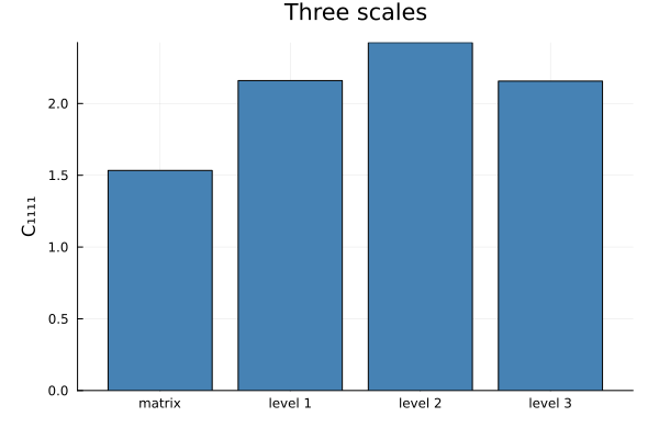
§5 Sensitivity across the scales
A nested lens addresses a scalar inside the inner cell, so a derivative of the outermost estimate with respect to an inner-scale modulus costs one forward-mode pass through the whole chain.
lens = nested(:M, :C, property(:matrix, :C, :μ))
idx = C -> get_array(C)[1, 2, 1, 2]
d_ad = derivative(outer, MoriTanaka(), lens; indexer = idx)
x₀ = get_param(outer, lens)
d_fd = (
    idx(homogenize(set_param(outer, lens, x₀ + 1.0e-6), MoriTanaka(), :C)) -
        idx(homogenize(set_param(outer, lens, x₀ - 1.0e-6), MoriTanaka(), :C))
) / 2.0e-6
@printf "\nd(outer μ)/d(inner matrix β) : AD %.10f   FD %.10f\n" d_ad d_fd
d(outer μ)/d(inner matrix β) : AD 1.0702098548 FD 1.0702098549The lenses an assembly answers are its own: radius_param and center_param for the geometry, property for the moduli. It has no amount — volume fractions are derived from the geometry and the cell size, so there is nothing to vary independently — and asking for one says so.
for lens in (amount(:p1), shape_param(:semi_axes))
    try
        get_param(inner, lens)
    catch e
        println("  ", nameof(typeof(lens)), " → ", first(split(sprint(showerror, e), ";")))
    end
end
AmountParameter → ArgumentError: ParticleAssembly: an assembly stores no amount: volume fractions are derived from the particle geometry and the cell size, so vary a radius (`radius_param`) or the boundary instead
DistributionShapeParameter → ArgumentError: ParticleAssembly: an assembly carries explicit positions rather than a distribution shape§6 The cost of an anisotropic reference
The isotropic interaction tensor is a closed form; the anisotropic one is a quadrature differentiated twice, so it is some three orders of magnitude dearer. That is the price of the chaining above, and it is why the dispatcher keeps the closed form whenever the reference is isotropic.
ia, ib, r = Ellipsoid(1.0), Ellipsoid(0.8), [0.0, 0.0, 4.0]
Cgen = Tens(get_array(C_m))
interaction_tensor(ia, ib, r, C_m); interaction_tensor(ia, ib, r, Cgen)   # warm up
t_iso = @elapsed for _ in 1:200
    interaction_tensor(ia, ib, r, C_m)
end
t_ani = @elapsed for _ in 1:20
    interaction_tensor(ia, ib, r, Cgen)
end
@printf "\nisotropic closed form : %8.1f µs\n" t_iso / 200 * 1.0e6
@printf "anisotropic multipole : %8.1f µs   (same values, generic type)\n" t_ani / 20 * 1.0e6
@printf "agreement             : %.2e\n" maximum(
    abs.(
        get_array(interaction_tensor(ia, ib, r, Cgen)) .-
            get_array(interaction_tensor(ia, ib, r, C_m))
    )
) / maximum(abs.(get_array(interaction_tensor(ia, ib, r, C_m))))

p_full = plot(p1; size = (700, 430))
p_full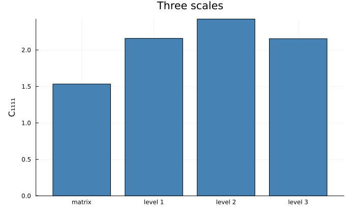
This page was generated using Literate.jl.