A fractured-reservoir well test

A synthetic fractured reservoir produced by a vertical well, in which the fracture apertures follow the effective stress and the permeability follows the apertures. The model, the microstructure and the two comparison cases are those of [71], § 3.2.

Everything here is three-dimensional and anisotropic: two vertical fracture families make the reservoir conduct six times better along than along , in a problem whose geometry and loading are both axisymmetric.

This page is static

Figures come from scripts/fe/arma2011_welltest.jl, run by hand and committed. A documentation build never runs a coupled reservoir simulation.

The microstructure

Solid phase   GPa,  ; matrix permeability , so the fractures carry the flow.

family	dip	dip azimuth	radius	aperture	conductivity	density
1	90°	22.5°	1 m	10⁻³ m	6.7·10⁻¹¹ m³	0.37
2	90°	157.5°	1 m	10⁻³ m	6.7·10⁻¹¹ m³	0.37

props = Dict(:C => C_SOLID, :K => TensISO{3}(1.0e-18))
rve = RVE()
add_phase!(rve, :M, Ellipsoid(1.0), props; fraction = :rest)
for φ in (π/8, 7π/8)                       # dip 90° ⇒ the normal is horizontal
    add_phase!(rve, gensym(), ConductiveCrack(1.0; conductivity = 6.7e-11,
               euler_angles = (π/2, φ)), props; density = 0.37)
end
mat = FracturedPoroelasticRock(rve, SelfConsistent(); ω₀ = (5.0e-4, 5.0e-4),
                               k_matrix = 1.0e-18)

One microstructure, every coefficient the coupled problem needs:

ℂʰᵒᵐ₃₃₃₃ = 3.189·10⁴ MPa
𝐁       = diag(0.9157, 0.7212, 0.4911)             anisotropic Biot tensor
1/M     = 2.837·10⁻⁵ MPa⁻¹
𝐊       = diag(9.66·10⁻¹², 5.63·10⁻¹¹, 5.81·10⁻¹¹) m²

Both families are vertical, so lies in both fracture planes and conducts most; bisects the two normals and conducts least. A density of 0.37 per family is past the percolation threshold of this network, which is why is set by the fracture conductivity and not by the matrix.

Geometry, mesh, and why a quarter is enough

A cylinder of radius 3500 m and height 200 m, produced along its axis. A fracture normal is defined up to a sign, so reflecting about maps the 22.5° family onto the 157.5° one, and so does reflecting about : the microstructure has both symmetry planes and a quarter model with rolling conditions is exact.

The radial layers are geometric (cylinder_sector_grid): the pressure drop is logarithmic in , so uniform layers would resolve nothing at the well and waste every element far from it.

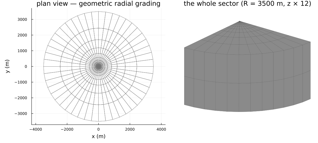
672 hexahedra, 4524 dofs	for
from 0.15 m to 3500 m	28 geometric layers
draw-down 24 h at   per meter of well	then shut in for 48 h

Prescribed flow rate on the well wall, no flow through the top and bottom faces,   on the outer boundary; rolling on the bottom and lateral boundaries, free top face.

The solve

The weak form, its backward-Euler discretization and the four tangent blocks are on the coupled poroelastic problem; the driver is thirty lines around mfh_poro_element! and knows nothing about fractures.

EXT.mfh_poro_element!(
    Ke, re, cvu, cvp, material, xe[URANGE], xe[PRANGE],
    states[cellid(cell)], states_old[cellid(cell)], Δt, mob[cellid(cell)];
    u_range = URANGE, p_range = PRANGE, cache = cache
)

Two models are compared, as in the reference:

M1	the homogenized properties are computed once and frozen
M2	apertures follow the Terzaghi effective stress, conductivities follow the cubic law, follows

Both share the same mechanics: for flat cracks is the   limit and carries no aperture, so as long as no family closes, , and are identical in M1 and M2. The two models differ through the permeability alone — which makes the comparison a clean measurement of the hydromechanical coupling.

The pressure field

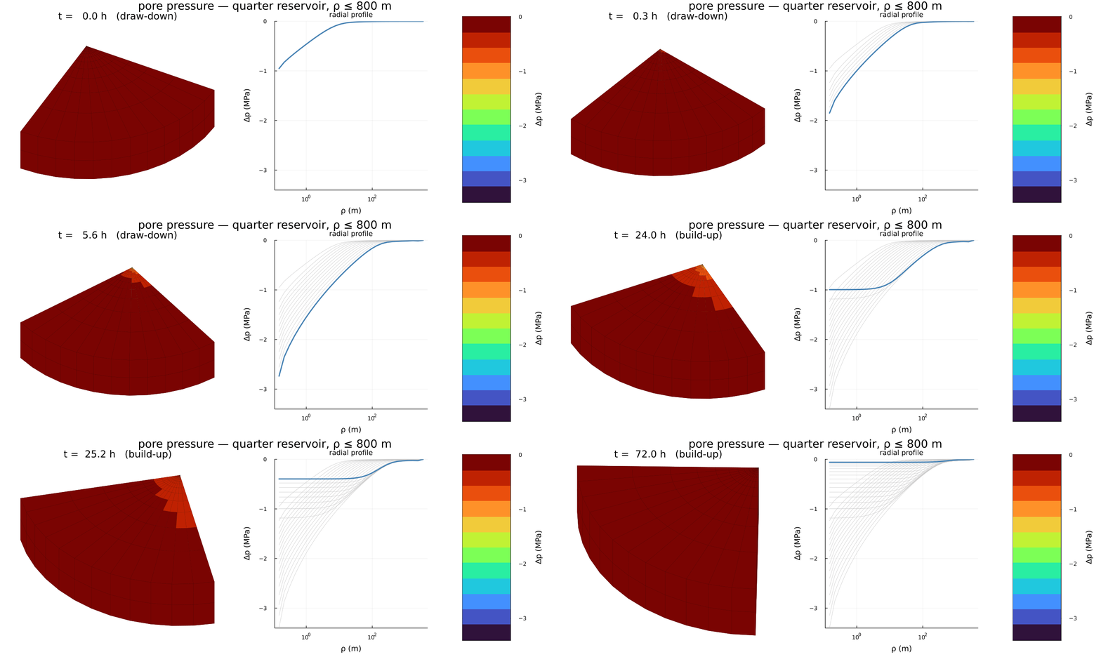
The isobars are elongated along , the direction the fracture network conducts best: an anisotropic microstructure printing itself on an axisymmetric problem.

Well pressure

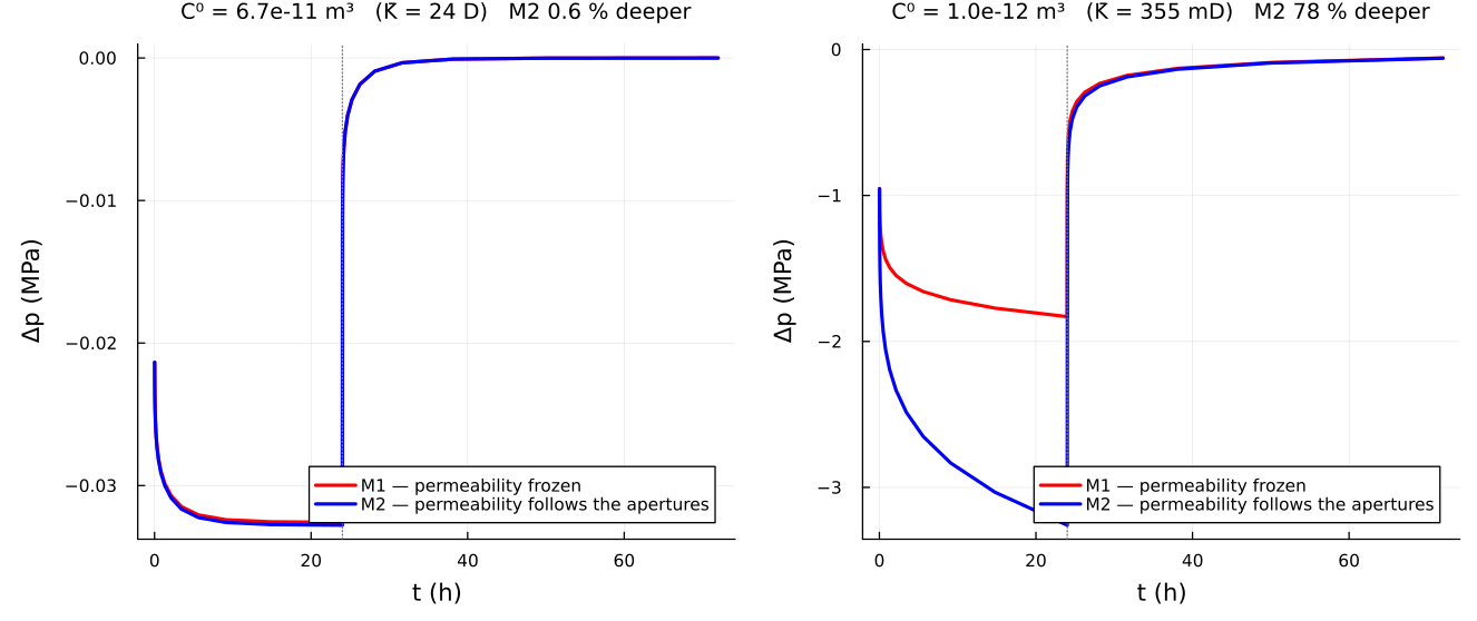
Pressure falls during the draw-down and recovers after the well is shut in; M2 draws down deeper than M1, because the pressure drop closes the fractures a little, the cubic law turns that into a conductivity drop, and a less permeable reservoir needs a larger draw-down to deliver the same rate. The build-up is far less sensitive.

Two cases, and why

Taking the table above literally, the permeability estimate used here gives a 23-darcy reservoir, a draw-down of 33 kPa and a 0.6 % gap between the two models — the left panel, which looks flat because it is flat. The published figures are an order of magnitude away: −1.8 MPa for M1 and a 33 % gap.

Steady radial flow gives  , so −1.8 MPa implies    — about 470 mD, consistent with the published permeability map. The estimate here returns  , ≈ 55 times larger, and that one number propagates linearly through the whole chain:

The right panel tests that reading directly: the fracture conductivity is calibrated to   mD — the knob § 1.3 of the reference leaves open, since may differ from the Poiseuille value "to account for tortuosity due to the roughness of fracture lips or to the fracture filling" — and nothing else is touched. Then

	M1 draw-down at 24 h	M2 vs M1	at the well face
here, calibrated	−1.83 MPa	+78 %	−70 %
published	−1.8 MPa	+33 %	≈ −50 %

M1 lands on the published value, and the draw-down is still declining at 24 h rather than stabilized, as published — the diffusion time scales as too. The coupling comes out about twice too strong: calibrating the conductivity fixes the permeability level, but not its sensitivity, and past percolation this estimate is very nearly proportional to , whereas the reference damps that response. Same mechanisms, same signs, an amplitude a factor two apart.

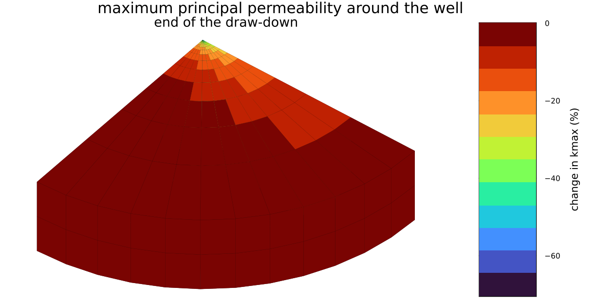
The permeability is reduced near the well, where the pressure variation is most negative, and the reduction is itself anisotropic — the isovalue bands are not circular.

What this reproduces, and what it does not

• Reproduced: the microstructure, the joint poroelastic and hydraulic upscaling from one RVE, the Terzaghi-driven aperture update, the cubic law, the coupled u–p simulation and both models — with the published draw-down magnitude once the permeability level is matched, and every qualitative conclusion of § 3.2.

• Not reproduced: the reference's self-consistent permeability, which carries a matrix concentration factor built on the order-2 Hill tensor of the effective medium. The estimate here reads each family's saturated contribution in the effective medium without that factor (fracture_permeability), so the two agree in structure — same percolation mechanism, same saturation — but differ by ≈ 55 on the level and ≈ 2 on the sensitivity. It is not transcribed here because the equations that define it are, in the copy at hand, not legible with enough confidence to implement without guessing.

• Not shipped: the consolidation column of § 3.1, models M1/M2/M3 — the case where a family actually closes during the loading. Everything it needs is here; see the roadmap.