Frequency or time? Three routes to the same viscoelastic composite

MeanFieldHomogenization reaches the effective behavior of a linear viscoelastic composite by three entirely separate roads:

• the frequency route — replace every modulus by its complex counterpart and call homogenize unchanged, as in the viscoelastic composites tutorial;

• the time route — homogenize_alv, which discretizes the Volterra operators on a time grid and never leaves the time domain, as in the ageing creep application;

• the Laplace-Carson route — homogenize_lc, which does the same and then inverts the answer back to the time domain numerically.

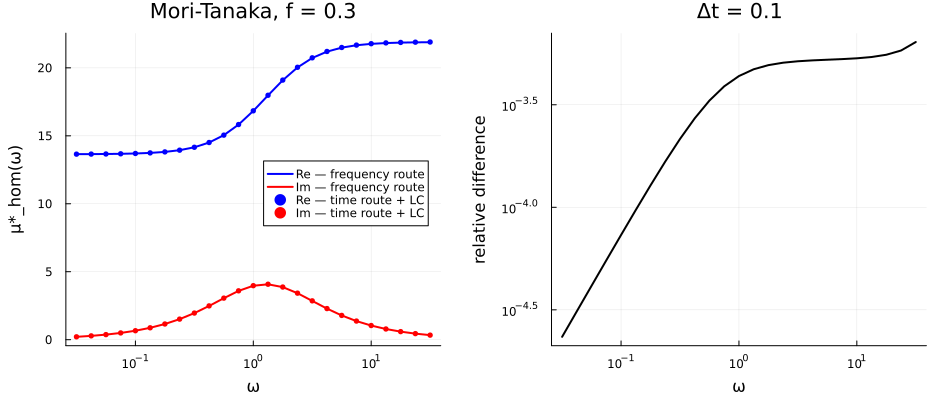
They share no code. For a non-ageing material the correspondence principle says all three must nevertheless agree, and this page checks that they do — quantitatively, and with each source of discrepancy identified rather than merely bounded.

Which way the transform runs

The forward direction is easy: the time route produces a sampled relaxation function , and its Laplace-Carson transform

is a plain quadrature. Evaluated at   it is exactly what the frequency route computes directly, and §4 compares the two that way.

The reverse direction — inverting the frequency answer back into the time domain — is genuinely ill-posed, which is why this page used to stop at two routes. It is now available: §6 runs it with inverse_carson and lands on the time route's own curve, so the comparison closes in both directions.

using MeanFieldHomogenization
using TensND
using LinearAlgebra
using QuadGK
using Printf
using Plots
gr()  # headless backend; GKSwstype is set to "100" before Literate runs

Plots.GRBackend()

§1 Two standard-solid phases

Each phase is a standard solid (Zener): a relaxation function decaying from an instantaneous modulus to a finite long-time modulus,

with the relaxed (long-time) shear modulus, the relaxing part, the shear relaxation time, and likewise in bulk. A finite keeps the composite from flowing indefinitely, so the relaxation function has a plateau that the truncated time grid can actually reach — the one requirement of the comparison below.

The Laplace-Carson transform of such a kernel is elementary,      , which is what feeds the frequency route.

A standard solid in each channel is zener_maxwell, and iso_rheology pairs the two into an isotropic fourth-order model. The point of describing the material this way is that one object serves all three routes: carson_relaxation(z, p) is the transformed stiffness the frequency and Laplace-Carson routes need, and ViscoLaw(z) is the time-domain kernel the ageing route needs. Nothing has to be written twice, so the three routes are guaranteed to be comparing the same material.

standard_solid(k∞, k_d, τk, μ∞, μ_d, τμ) =
    iso_rheology(zener_maxwell(k∞, k_d, τk), zener_maxwell(μ∞, μ_d, τμ))

const Z_MATRIX = standard_solid(30.0, 20.0, 1.0, 10.0, 8.0, 0.7)
const Z_INCL = standard_solid(80.0, 10.0, 2.0, 30.0, 5.0, 1.5)
const F_INCL = 0.3

0.3

§2 The frequency route

Nothing viscoelastic happens here: an RVE of ComplexF64 moduli goes through the ordinary Mori-Tanaka scheme, and the effective shear modulus is read off the result.

function mu_frequency(ω)
    p = im * ω
    rve = RVE()
    add_phase!(rve, :M, Ellipsoid(1.0), Dict(:C => carson_relaxation(Z_MATRIX, p)); fraction = :rest)
    add_phase!(
        rve, :I, Ellipsoid(1.0), Dict(:C => carson_relaxation(Z_INCL, p));
        fraction = F_INCL
    )
    return TensND.get_data(homogenize(rve, MoriTanaka()))[2] / 2
end

mu_frequency (generic function with 1 method)

§3 The time route, and how to read a relaxation function out of it

homogenize_alv returns the effective operator as a   block matrix acting on a strain history sampled on the grid — the trapezoidal representation of the Stieltjes integral    ([60]). Its blocks are differences of kernel values, not kernel values, so reading off a column would be wrong.

The physical extraction is a relaxation test. Applying a unit strain step at   means a history vector whose every time slot holds the same strain, so the stress at is the row sum:

iso_params_from_blocks splits the block matrix into its two isotropic parts   and  , so the row sums of give directly.

function mu_relaxation(times)
    rve = RVE()
    add_phase!(rve, :M, Ellipsoid(1.0), Dict(:C => ViscoLaw(Z_MATRIX)); fraction = :rest)
    add_phase!(
        rve, :I, Ellipsoid(1.0), Dict(:C => ViscoLaw(Z_INCL));
        fraction = F_INCL
    )
    R̃ = homogenize_alv(rve, MoriTanaka(), :C; times = times)
    _, β = iso_params_from_blocks(R̃)
    return vec(sum(β, dims = 2)) ./ 2      # 2μ(tᵢ) → μ(tᵢ)
end

times = collect(range(0.0, 40.0; length = 401))
μ_t = mu_relaxation(times)

@printf(
    "μ_hom(0) = %.5f  (instantaneous)      μ_hom(T = %.0f) = %.5f  (relaxed)\n",
    μ_t[1], times[end], μ_t[end]
)

μ_hom(0) = 21.90109  (instantaneous)      μ_hom(T = 40) = 13.64486  (relaxed)

The grid must be long enough for the plateau to be reached: the tail beyond is then a constant, and its contribution to the transform is the closed form   rather than a truncation error.

function mu_from_time(ω, times, μ_t)
    p = im * ω
    interp(t) = begin
        i = searchsortedlast(times, t)
        i ≥ length(times) && return μ_t[end]
        θ = (t - times[i]) / (times[i + 1] - times[i])
        (1 - θ) * μ_t[i] + θ * μ_t[i + 1]
    end
    I, _ = quadgk(t -> interp(t) * exp(-p * t), times[1], times[end]; rtol = 1.0e-11)
    return p * I + μ_t[end] * exp(-p * times[end])
end

mu_from_time (generic function with 1 method)

§4 The comparison

ωs = exp10.(range(-1.5, 1.5; length = 25))
μ_freq = [mu_frequency(ω) for ω in ωs]
μ_time = [mu_from_time(ω, times, μ_t) for ω in ωs]
rel_err = abs.(μ_freq .- μ_time) ./ abs.(μ_freq)

@printf("\n   ω      Re μ* (freq)  Re μ* (time)  Im μ* (freq)  Im μ* (time)   rel. err\n")
for i in 1:4:length(ωs)
    @printf(
        "%7.3f   %11.5f  %12.5f  %12.5f  %12.5f   %.2e\n",
        ωs[i], real(μ_freq[i]), real(μ_time[i]),
        imag(μ_freq[i]), imag(μ_time[i]), rel_err[i]
    )
end

p1 = plot(
    ωs, real.(μ_freq); xscale = :log10, lw = 2, color = :blue,
    label = "Re — frequency route", xlabel = "ω", ylabel = "μ*_hom(ω)",
    title = "Mori-Tanaka, f = $F_INCL", legend = :right,
)
plot!(p1, ωs, imag.(μ_freq); lw = 2, color = :red, label = "Im — frequency route")
scatter!(p1, ωs, real.(μ_time); marker = :circle, ms = 3, color = :blue,
    markerstrokewidth = 0, label = "Re — time route + LC")
scatter!(p1, ωs, imag.(μ_time); marker = :circle, ms = 3, color = :red,
    markerstrokewidth = 0, label = "Im — time route + LC")

p2 = plot(
    ωs, rel_err; xscale = :log10, yscale = :log10, lw = 2, color = :black,
    xlabel = "ω", ylabel = "relative difference", legend = false,
    title = "Δt = $(round(times[2] - times[1], digits = 3))",
)
plt = plot(
    p1, p2; layout = (1, 2), size = (950, 400),
    left_margin = 5Plots.mm, bottom_margin = 5Plots.mm,
)

§5 The difference is the time step, and nothing else

The two routes do not agree exactly, and they should not: the time route integrates the Volterra operator with the trapezoidal rule. Halving should therefore divide the discrepancy by four — which is a much stronger statement than a single small number, because it identifies what the remaining difference is.

@printf("\n   Δt        relative difference at ω = 1\n")
prev = NaN
for npts in (101, 201, 401)
    tg = collect(range(0.0, 40.0; length = npts))
    e = abs(mu_from_time(1.0, tg, mu_relaxation(tg)) - mu_frequency(1.0)) / abs(mu_frequency(1.0))
    ratio = isnan(prev) ? "" : @sprintf("   (÷ %.2f)", prev / e)
    @printf("%7.3f     %.3e%s\n", tg[2] - tg[1], e, ratio)
    global prev = e
end

   Δt        relative difference at ω = 1
  0.400     6.956e-03
  0.200     1.745e-03   (÷ 3.99)
  0.100     4.366e-04   (÷ 4.00)

The factor is 4 to two digits: the entire gap between the frequency and the time route is the trapezoidal error, and the two implementations agree in the continuum limit.

§6 The third route: inverting the frequency answer

Everything so far ran the transform the easy way. The reverse direction is now available too: homogenize_lc evaluates the same Mori-Tanaka estimate at the Carson variables an inversion algorithm asks for, and hands back directly.

Note what is not needed: no time grid, no Volterra operator, no trapezoidal rule. The answer at t = 7 costs a couple of dozen elastic homogenizations and nothing else, whereas the time route has to march the whole history up to t = 7 to get there.

function cell_lc(p)
    rve = RVE()
    add_phase!(rve, :M, Ellipsoid(1.0), Dict(:C => carson_relaxation(Z_MATRIX, p)); fraction = :rest)
    add_phase!(
        rve, :I, Ellipsoid(1.0), Dict(:C => carson_relaxation(Z_INCL, p));
        fraction = F_INCL
    )
    return rve
end

probe_times = [0.05, 0.2, 1.0, 3.0, 10.0, 30.0]
μ_lc = [
    TensND.get_data(C)[2] / 2
        for C in homogenize_lc(cell_lc, MoriTanaka(), :C; times = probe_times)
]

6-element Vector{Float64}:
 21.389490542752515
 20.0403983789771
 15.981237365750689
 13.858997536906973
 13.645327614503294
 13.64485981576824

The three inversion algorithms should agree with each other far more closely than any of them agrees with the discretized time route, because they are approximating the same exact quantity while the time route approximates a different one.

μ_lc_gs = [
    TensND.get_data(C)[2] / 2
        for C in homogenize_lc(
        cell_lc, MoriTanaka(), :C; times = probe_times, method = GaverStehfest(16)
    )
]
μ_lc_dh = [
    TensND.get_data(C)[2] / 2
        for C in homogenize_lc(
        cell_lc, MoriTanaka(), :C; times = probe_times, method = DeHoog()
    )
]

interp_time(t) = begin
    i = clamp(searchsortedlast(times, t), 1, length(times) - 1)
    θ = (t - times[i]) / (times[i + 1] - times[i])
    (1 - θ) * μ_t[i] + θ * μ_t[i + 1]
end

@printf("\n     t     μ (time route)   μ (LC/Talbot)   LC/GS − Talbot   LC/deHoog − Talbot   time − LC\n")
for (i, t) in enumerate(probe_times)
    @printf(
        "%7.2f   %13.7f   %13.7f   %14.2e   %18.2e   %9.2e\n",
        t, interp_time(t), μ_lc[i],
        abs(μ_lc_gs[i] - μ_lc[i]) / μ_lc[i],
        abs(μ_lc_dh[i] - μ_lc[i]) / μ_lc[i],
        abs(interp_time(t) - μ_lc[i]) / μ_lc[i]
    )
end

     t     μ (time route)   μ (LC/Talbot)   LC/GS − Talbot   LC/deHoog − Talbot   time − LC
   0.05      21.4057296      21.3894905         7.85e-08             9.18e-10    7.59e-04
   0.20      20.0406996      20.0403984         7.20e-09             7.97e-10    1.50e-05
   1.00      15.9818190      15.9812374         2.88e-08             7.89e-10    3.64e-05
   3.00      13.8591454      13.8589975         3.34e-06             9.83e-10    1.07e-05
  10.00      13.6453266      13.6453276         1.73e-06             9.37e-10    7.74e-08
  30.00      13.6448598      13.6448598         1.15e-06             1.00e-09    2.76e-13

The last three columns are the point of the whole page. Reading them right to left:

• time − LC is the trapezoidal error of the time route on this grid — the same quantity §5 showed converging at order 2. It is by far the largest discrepancy (8e-4 at t = 0.05) and it is a property of the time route alone. It shrinks to 3e-13 by t = 30, not because the quadrature improves but because the relaxation function has reached its plateau and there is nothing left to integrate badly.

• LC/deHoog − Talbot, a flat 1e-9 across five decades of time, is the inversion error. Two completely different quadratures — a Hankel contour and an accelerated Fourier series on a Bromwich line — landing on the same number to nine digits is a strong statement that both have converged.

• LC/GS − Talbot, between 1e-8 and 3e-6, is GaverStehfest's own budget: it buys five to eight digits instead of twelve, in exchange for evaluating the scheme at real p only, which keeps the whole sweep in real arithmetic.

So the errors separate cleanly and each is attributable — which is a far more useful statement than "the three routes agree to a millesimal", and a much better test: a regression in any one of the three would move exactly one column.

# Log time axis: the whole relaxation happens in the first two decades, and a
# linear axis would pile every probe point against the left edge.
p3 = plot(
    times[2:end], μ_t[2:end];
    xscale = :log10, lw = 2, color = :black,
    label = "time route (ALV, Δt = $(round(times[2] - times[1], digits = 3)))",
    xlabel = "t", ylabel = "μ_hom(t)", legend = :topright,
    title = "Back in the time domain, three ways"
)
scatter!(
    p3, probe_times, μ_lc;
    marker = :circle, ms = 7, color = :crimson, markerstrokewidth = 0,
    label = "Laplace-Carson + FixedTalbot"
)
scatter!(
    p3, probe_times, μ_lc_gs;
    marker = :diamond, ms = 5, color = :seagreen, markerstrokewidth = 0,
    label = "…+ GaverStehfest (real p)"
)

p4 = plot(
    probe_times, abs.(μ_lc_dh .- μ_lc) ./ μ_lc;
    xscale = :log10, yscale = :log10, lw = 2, marker = :circle, color = :royalblue,
    label = "inversion error (deHoog vs Talbot)",
    xlabel = "t", ylabel = "relative difference", legend = :right,
    title = "the two error sources, separated"
)
plot!(
    p4, probe_times, abs.(μ_lc_gs .- μ_lc) ./ μ_lc;
    lw = 2, marker = :diamond, color = :seagreen, label = "GaverStehfest budget"
)
plot!(
    p4, probe_times, [abs(interp_time(t) - μ_lc[i]) / μ_lc[i] for (i, t) in enumerate(probe_times)];
    lw = 2, marker = :square, color = :black, label = "trapezoidal error of the time route"
)

plt3 = plot(
    p3, p4; layout = (1, 2), size = (1050, 420),
    left_margin = 5Plots.mm, bottom_margin = 5Plots.mm
)
plt3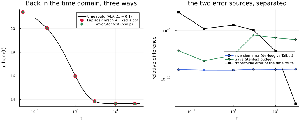

This only works because the material does not age

Both transform routes need to depend on   alone. When a phase solidifies progressively, and enter independently, the Laplace-Carson transform no longer factorizes the convolution, and two of the three routes simply cease to exist — which is why homogenize_alv is not a redundant implementation. See the ageing creep application for a case where only the time route applies.

---

This page was generated using Literate.jl.