Choosing a numerical Laplace inversion

Going from a relaxation function to its Laplace-Carson transform is a quadrature — easy, stable, and what the frequency-or-time comparison does. Coming back is the ill-posed direction: the transform smooths, so undoing it amplifies whatever is left of the arithmetic.

MeanFieldHomogenization ships four algorithms for it. None of them is best everywhere, and the differences between them are large — five orders of magnitude on the same problem — so this page measures rather than asserts.

All four are written to be generic in the number type, which is why ForwardDiff traverses them (§4) and why working in BigFloat actually buys precision (§2).

using MeanFieldHomogenization
using ForwardDiff
using SpecialFunctions
using Printf
using Plots
gr()  # headless backend; GKSwstype is set to "100" before Literate runs

METHODS = [
    ("Gaver-Stehfest (16)", GaverStehfest(16), :seagreen),
    ("fixed Talbot (24)", FixedTalbot(24), :crimson),
    ("Talbot-Trefethen (24)", TalbotTrefethen(24), :darkorange),
    ("de Hoog (16)", DeHoog(), :royalblue),
]

4-element Vector{Tuple{String, AbstractLaplaceInversion, Symbol}}:
 ("Gaver-Stehfest (16)", GaverStehfest(16), :seagreen)
 ("fixed Talbot (24)", FixedTalbot(24), :crimson)
 ("Talbot-Trefethen (24)", TalbotTrefethen(24, 0.0), :darkorange)
 ("de Hoog (16)", DeHoog(16, nothing, 1.0e-9), :royalblue)

§1 Four transforms with known inverses

The four test pairs are chosen to separate the algorithms rather than to flatter them:

transform	inverse	what it probes
		the ordinary decaying case
		algebraic growth, a pole of order 3 at the origin
		a branch cut along the negative real axis
		oscillation, which is what actually separates them

PAIRS = [
    ("1/(p+2)  ↔  e^{-2t}", p -> 1 / (p + 2), t -> exp(-2t)),
    ("1/p³  ↔  t²/2", p -> 1 / p^3, t -> t^2 / 2),
    ("1/√p  ↔  1/√(πt)", p -> 1 / sqrt(p), t -> 1 / sqrt(π * t)),
    ("1/(p²+9)  ↔  sin(3t)/3", p -> 1 / (p^2 + 9), t -> sin(3t) / 3),
]

ts = exp10.(range(-1, 0.8; length = 60))

panels = map(PAIRS) do (title, F, f)
    plt = plot(
        xscale = :log10, yscale = :log10, xlabel = "t",
        ylabel = "relative error", title = title, legend = :bottomright,
        ylims = (1.0e-16, 10)
    )
    for (name, m, col) in METHODS
        err = [max(abs(inverse_laplace(F, t, m) - f(t)) / abs(f(t)), 1.0e-16) for t in ts]
        plot!(plt, ts, err; lw = 2, color = col, label = name)
    end
    plt
end
p_pairs = plot(panels...; layout = (2, 2), size = (1100, 750))
p_pairs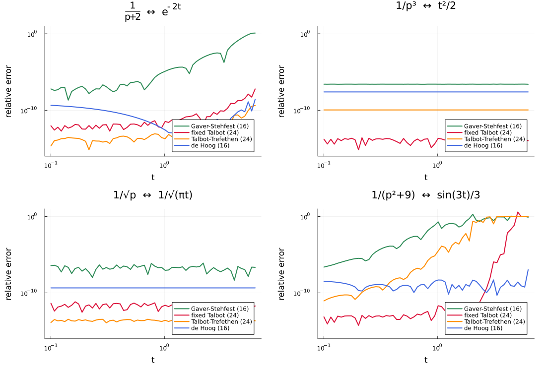

Two conclusions worth stating plainly, because both contradict what one might expect:

Branch cuts are not a problem for the Talbot family. Their contour is Hankel-shaped: it wraps around the negative real axis rather than crossing it, which is precisely how Talbot quadratures were designed to handle singularities there. 1/\sqrt{p} inverts at 1e-12. Every fractional model in the catalog — ScottBlair, HuetSayegh, Model2S2P1D — is in the same situation.

Oscillation is what separates them. Gaver-Stehfest, whose nodes are all real, has no way to see a rotating phase and returns O(1) error; Talbot-Trefethen, whose contour is tuned for decay, is not much better. Only FixedTalbot and DeHoog hold up.

for (title, F, f) in PAIRS
    @printf "%-24s " title
    for (name, m, _) in METHODS
        @printf "%s=%.1e  " first(split(name)) (abs(inverse_laplace(F, 1.0, m) - f(1.0)) / abs(f(1.0)))
    end
    println()
end

1/(p+2)  ↔  e^{-2t}      Gaver-Stehfest=1.1e-05  fixed=2.6e-12  Talbot-Trefethen=2.0e-14  de=3.1e-13
1/p³  ↔  t²/2            Gaver-Stehfest=2.6e-07  fixed=1.0e-14  Talbot-Trefethen=1.1e-10  de=2.5e-08
1/√p  ↔  1/√(πt)         Gaver-Stehfest=7.2e-08  fixed=2.6e-12  Talbot-Trefethen=2.5e-14  de=4.5e-10
1/(p²+9)  ↔  sin(3t)/3   Gaver-Stehfest=1.4e-01  fixed=1.5e-12  Talbot-Trefethen=7.3e-06  de=4.6e-09

§2 More terms is not more accurate

Gaver-Stehfest sums weights that alternate in sign with magnitudes up to times the answer, so it needs roughly 2.3 M digits of working precision to return M correct ones. In Float64 that puts the optimum at N = 14–16 and makes everything beyond N ≈ 18 worse.

The weights themselves are exact — they are cached as Rational{BigInt} and converted to the working type on demand — so the ceiling really is the arithmetic and not the coefficients. Running the same N in BigFloat proves it.

Ns = 4:2:34
err_f64 = [abs(inverse_laplace(p -> 1 / (p + 2), 1.0, GaverStehfest(N)) - exp(-2.0)) / exp(-2.0) for N in Ns]
err_big = setprecision(256) do
    [
        Float64(
            abs(
                inverse_laplace(p -> 1 / (p + big(2)), big(1.0), GaverStehfest(N)) -
                    exp(big(-2.0))
            ) / exp(big(-2.0))
        ) for N in Ns
    ]
end

p_terms = plot(
    Ns, max.(err_f64, 1.0e-17);
    yscale = :log10, lw = 2.5, marker = :circle, color = :seagreen,
    label = "Float64", xlabel = "N", ylabel = "relative error",
    title = "Gaver-Stehfest: the optimum, and past it", legend = :bottomleft
)
plot!(p_terms, Ns, max.(err_big, 1.0e-17); lw = 2.5, marker = :square, color = :purple, label = "BigFloat (256 bits)")
vline!(p_terms, [16]; color = :grey, ls = :dash, label = "the Float64 default, N = 16")

@printf "best Float64 : N = %d, error %.2e\n" Ns[argmin(err_f64)] minimum(err_f64)
@printf "at N = 34    : Float64 %.2e   BigFloat %.2e\n" err_f64[end] err_big[end]

best Float64 : N = 18, error 2.27e-06
at N = 34    : Float64 1.35e+05   BigFloat 1.39e-14

§3 Cost, and why DeHoog exists

Each inversion costs N evaluations of the transform — 16 for Gaver-Stehfest, 24 for the Talbot pair, 2N+1 = 33 for de Hoog. When the transform is a formula that hardly matters. When it is a homogenization scheme, as in homogenize_lc, it is the whole cost of the computation.

De Hoog's nodes do not depend on t, so one node set can serve several times at once. What limits the sharing is that its accuracy depends on the ratio t/T alone, and collapses below t/T ≈ 0.05. The default therefore splits a grid into blocks spanning a factor of three and gives each block its own node set — uniform accuracy, at a fraction of the per-point cost.

grid = exp10.(range(-3, 3; length = 40))
exact_grid = exp.(-grid)
blocked = inverse_laplace(p -> 1 / (p + 1), grid, DeHoog())
shared = inverse_laplace(p -> 1 / (p + 1), grid, DeHoog(; T = 2 * maximum(grid)))

p_blocks = plot(
    grid, max.(abs.(blocked .- exact_grid), 1.0e-18);
    xscale = :log10, yscale = :log10, lw = 2.5, color = :royalblue,
    label = "blocked by scale (the default)",
    xlabel = "t", ylabel = "absolute error", legend = :bottomleft,
    title = "de Hoog on a 6-decade grid"
)
plot!(p_blocks, grid, max.(abs.(shared .- exact_grid), 1.0e-18); lw = 2.5, ls = :dash, color = :grey, label = "one shared node set")

n_blocks = length(unique(map(t -> floor(log(3.3, t / minimum(grid))), grid)))
@printf "40 times over 6 decades: ~%d blocks × 33 = ~%d transform evaluations\n" n_blocks (33n_blocks)
@printf "  per-point instead    : 40 × 33 = %d\n" (40 * 33)

┌ Warning: DeHoog: some times fall below t/T = 0.15, where the continued-fraction acceleration loses most of its digits. Smallest t/T requested = 5.0e-7. Pass `T = nothing` to let the grid be split into scale blocks, or restrict `T` to the narrow window you actually need.
└ @ MeanFieldHomogenization.Viscoelasticity ~/work/MeanFieldHomogenization.jl/MeanFieldHomogenization.jl/src/Viscoelasticity/laplace_inversion.jl:780
40 times over 6 decades: ~12 blocks × 33 = ~396 transform evaluations
  per-point instead    : 40 × 33 = 1320

§4 Differentiating through an inversion

Every method here takes t::Real rather than t::AbstractFloat, computes its working type from the arguments, and never seeds an accumulator with zero. Those three things together are what let a ForwardDiff.Dual — or a Complex{Dual}, on the contour methods — pass through untouched.

The example below differentiates the inverse transform of    with respect to τ, against the exact  .

Rstar(τ, p) = 2.0 + 3.0 * p * τ / (1 + p * τ)
dR_exact(τ, t) = 3.0 * t * exp(-t / τ) / τ^2

τ0 = 1.5
p_ad = plot(
    xscale = :log10, yscale = :log10, xlabel = "t",
    ylabel = "relative error on ∂R/∂τ", legend = :bottomright,
    title = "ForwardDiff through the inversion", ylims = (1.0e-16, 1.0e-2)
)
for (name, m, col) in METHODS
    err = [
        max(
            abs(
                ForwardDiff.derivative(τ -> inverse_carson(p -> Rstar(τ, p), t, m), τ0) -
                    dR_exact(τ0, t)
            ) / abs(dR_exact(τ0, t)), 1.0e-16
        ) for t in ts
    ]
    plot!(p_ad, ts, err; lw = 2, color = col, label = name)
end
p_ad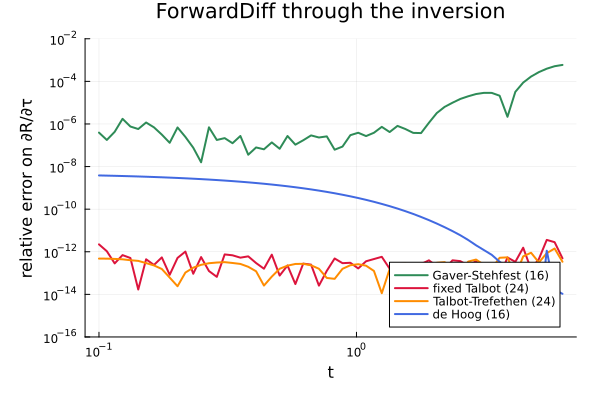

The gradients carry the same accuracy as the values themselves — the inversion is a linear combination of transform values, so the partials ride along the same sum.

For the time derivative specifically there is also a shortcut that needs no autodiff at all. Since   , the rate is an ordinary inverse transform of a shifted transform, which is what inverse_carson_rate does:

for (name, m, _) in METHODS
    d_ad = ForwardDiff.derivative(t -> inverse_carson(p -> Rstar(τ0, p), t, m), 0.8)
    d_id = inverse_carson_rate(p -> Rstar(τ0, p), 0.8, m; f_glassy = 5.0)
    exact = -3.0 / τ0 * exp(-0.8 / τ0)
    @printf "%-24s ∂/∂t by AD: %.2e   by the identity: %.2e\n" name (abs(d_ad - exact) / abs(exact)) (abs(d_id - exact) / abs(exact))
end

Gaver-Stehfest (16)      ∂/∂t by AD: 1.34e-07   by the identity: 3.20e-06
fixed Talbot (24)        ∂/∂t by AD: 6.48e-13   by the identity: 4.11e-13
Talbot-Trefethen (24)    ∂/∂t by AD: 9.84e-15   by the identity: 1.76e-14
de Hoog (16)             ∂/∂t by AD: 1.20e-10   by the identity: 1.19e-10

§5 What to reach for

	nodes	per inversion	use it when
FixedTalbot	complex	24	the default — best on every kernel tested
GaverStehfest	real	16	the transform must stay real: a whole homogenize_lc sweep in real arithmetic, and the only way to use SelfConsistent(algorithm = NewtonDefault()) there
DeHoog	complex	33, shared across a block of times	a multi-decade grid whose every point is a homogenization
TalbotTrefethen	complex	24	cross-checking against the ECHOES reference, or poles in the right half-plane

p_full = plot(
    p_pairs, plot(p_terms, p_blocks, p_ad; layout = (1, 3));
    layout = grid_layout = @layout([a{0.62h}; b]), size = (1400, 1150),
    left_margin = 6Plots.mm, bottom_margin = 6Plots.mm
)
p_full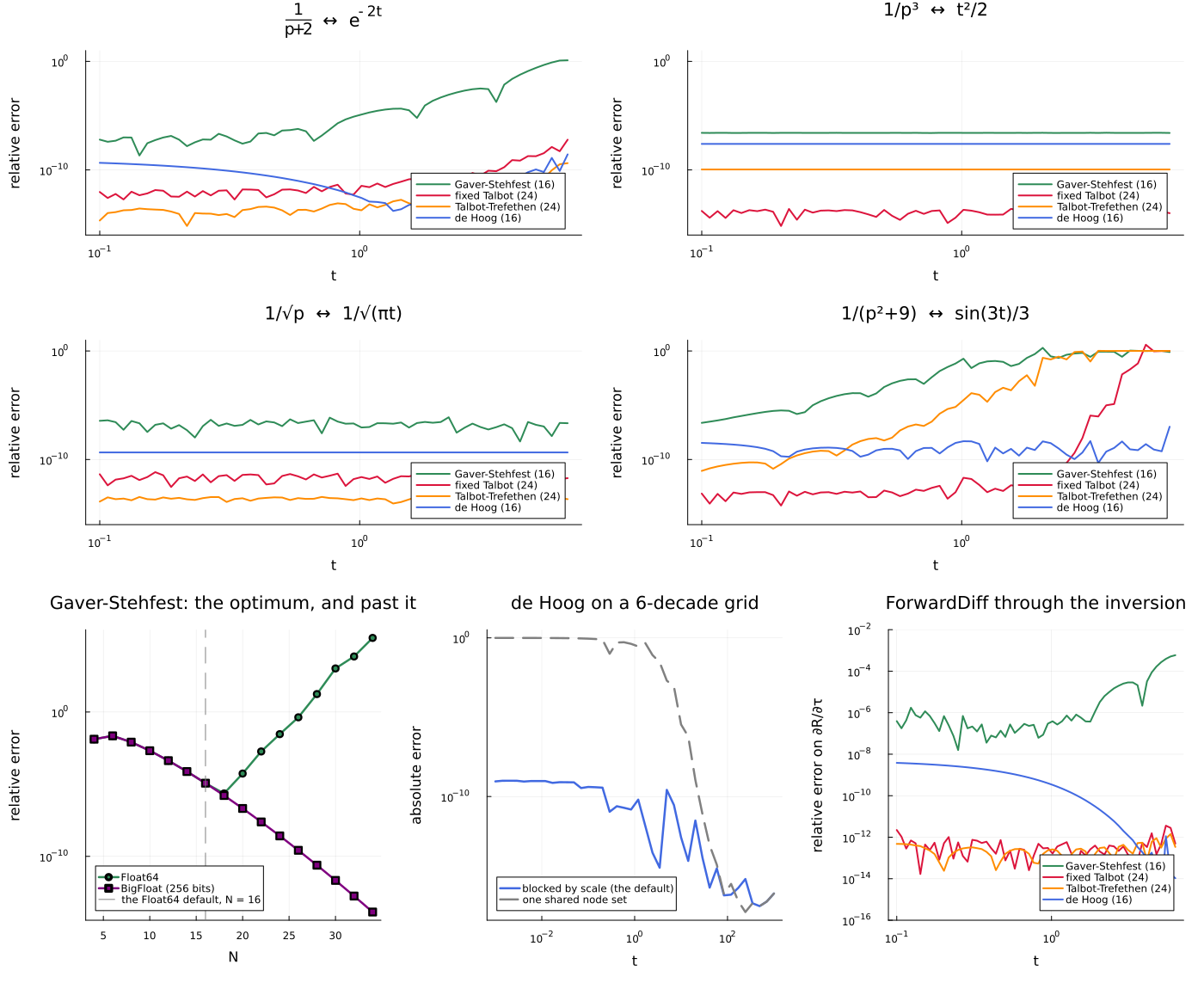

---

This page was generated using Literate.jl.