Crack distributions: isotropic or parallel

The same cracks, the same crack density, two orientation distributions — and two different effective media. This is the shortest example that exercises the three things a cracked RVE needs: a density instead of a volume fraction, an orientation distribution, and a scheme that can cope with a phase of zero volume.

The material is a solid of  ,   carrying penny-shaped cracks of density  . Everything below is cross-checked against values captured from a run of Echoes 1.0 on the same problem.

The two microstructures

The realizations are drawn with a fixed seed, so the two pictures differ only in the orientation rule — the crack positions are the same.

using MeanFieldHomogenization
using TensND
using LinearAlgebra
using Printf
using Plots
gr()

# Interactive-3-D helpers; `pkgdir` rather than `@__DIR__` so the include also
# resolves inside a Documenter `@example` block.
include(joinpath(pkgdir(MeanFieldHomogenization), "scripts", "common", "docviz.jl"))

const E₀, ν₀ = 1.0, 0.2
const C₀ = iso_stiffness_E_nu(E₀, ν₀)
const ε = 0.6
const k₀, μ₀ = k_mu(C₀)

@printf "intact solid : k = %.6f   μ = %.6f\n" k₀ μ₀

intact solid : k = 0.555556   μ = 0.416667

An isotropic distribution: every orientation equally likely, so the effective medium is isotropic however anisotropic each single crack is.

plotly_scene(
    rve_traces(; n = 70, semi_axes = (0.10, 0.10, 0.004), seed = 2024);
    uid = "cd-rve-iso", height = 470,
    title = "Isotropic distribution of penny cracks"
)

Parallel cracks: one common normal, here the direction of spherical angles  . The effective medium is transversely isotropic about that normal.

const n̂ = (sin(π / 4) * cos(π / 3), sin(π / 4) * sin(π / 3), cos(π / 4))

plotly_scene(
    rve_traces(; n = 70, semi_axes = (0.10, 0.10, 0.004), seed = 2024,
        orientation = n̂);
    uid = "cd-rve-aligned", height = 470,
    title = "Parallel cracks, all normals along n̂ = (√2/4, √6/4, √2/2)"
)

Building the two RVEs

A crack phase differs from an inclusion phase in two places only: it is declared with density instead of fraction, and its property dictionary carries the matrix stiffness — the crack-opening machinery needs the medium the crack opens in, not a stiffness of its own (a crack has none).

The orientation distribution is the symmetrize keyword. IsoSymmetrize() performs the exact SO(3) average of the concentration tensor; leaving it out keeps the single orientation carried by the crack's own frame.

function rve_isotropic(ε)
    r = RVE()
    add_phase!(r, :SOLID, Spheroid(1.0), Dict(:C => C₀); fraction = :rest)
    add_phase!(
        r, :CRACK, PennyCrack(1.0), Dict(:C => C₀);
        density = ε, symmetrize = IsoSymmetrize()
    )
    return r
end

function rve_parallel(ε; angles = (π / 4, π / 3))
    r = RVE()
    add_phase!(r, :SOLID, Spheroid(1.0), Dict(:C => C₀); fraction = :rest)
    add_phase!(
        r, :CRACK, PennyCrack(1.0; euler_angles = angles), Dict(:C => C₀);
        density = ε
    )
    return r
end

# The two angles of `euler_angles` are read here as the polar and azimuthal
# angles of the crack normal, which is the third column of the crack frame.
crack = PennyCrack(1.0; euler_angles = (π / 4, π / 3))
normal = [TensND.vecbasis(crack.basis, :cov)[i, 3] for i in 1:3]
@printf "crack normal : (%.6f, %.6f, %.6f)\n" normal...

crack normal : (0.353553, 0.612372, 0.707107)

Isotropic distribution

Three schemes, and they do not merely differ in value — they differ in behavior. MoriTanaka and DiluteDual coincide exactly here: a crack has no volume, so the Mori-Tanaka denominator reduces to the identity and the scheme collapses onto the dilute compliance estimate. That is not a bug, it is what the crack limit does to the algebra.

const SC = SelfConsistent(; abstol = 1.0e-8, maxiters = 400, select_best = true)
const ASC = AsymmetricSelfConsistent(; abstol = 1.0e-8, maxiters = 400, select_best = true)

kμ_iso(rve, scheme) = k_mu(best_fit_iso(homogenize(rve, scheme, :C)))

for (name, scheme) in (("Mori-Tanaka", MoriTanaka()), ("DiluteDual", DiluteDual()),
        ("SelfConsistent", SC), ("Asym. SC", ASC))
    k, μ = kμ_iso(rve_isotropic(ε), scheme)
    @printf "%-16s : k = %.6f   μ = %.6f   (3k, 2μ) = (%.6f, %.6f)\n" name k μ 3k 2μ
end

Mori-Tanaka      : k = 0.205255   μ = 0.218125   (3k, 2μ) = (0.615764, 0.436249)
DiluteDual       : k = 0.205255   μ = 0.218125   (3k, 2μ) = (0.615764, 0.436249)
SelfConsistent   : k = 0.133754   μ = 0.139589   (3k, 2μ) = (0.401262, 0.279179)
Asym. SC         : k = 0.000000   μ = 0.000000   (3k, 2μ) = (0.000000, 0.000000)

Against Echoes 1.0 at the same density. Echoes reports an isotropic tensor through its two Walpole coefficients , which is what the last column above prints:

echoes_iso = Dict(                    # captured from a run of Echoes 1.0
    "MT" => (k = 0.205254, μ = 0.218124),
    "SC" => (k = 0.133754, μ = 0.139589),
)

for (name, scheme) in (("MT", MoriTanaka()), ("SC", SC))
    k, μ = kμ_iso(rve_isotropic(ε), scheme)
    ref = echoes_iso[name]
    @printf "%s : Δk = %.2e   Δμ = %.2e\n" name abs(k - ref.k) abs(μ - ref.μ)
end

MT : Δk = 5.16e-07   Δμ = 7.09e-07
SC : Δk = 1.64e-08   Δμ = 2.83e-07

Both agree to the last captured digit. Note that it is the symmetric SelfConsistent that matches Echoes' SC on cracks, not AsymmetricSelfConsistent: the two solve different fixed points, and the next section is where that becomes visible.

Two self-consistent forms, two percolation thresholds

SelfConsistent iterates on the stiffness, AsymmetricSelfConsistent on the compliance. Both percolate — the effective moduli reach zero at a finite crack density, unlike Mori-Tanaka, which only decays asymptotically — but they do so at different densities, and that is the practical difference between them. The compliance form gives up first.

εs = range(0.0, 1.3; length = 131)
curves = Dict(
    "Mori-Tanaka" => [kμ_iso(rve_isotropic(e), MoriTanaka()) for e in εs],
    "SelfConsistent" => [kμ_iso(rve_isotropic(e), SC) for e in εs],
    "Asym. SC" => [kμ_iso(rve_isotropic(e), ASC) for e in εs],
)

Dict{String, Vector{Tuple{Float64, Float64}}} with 3 entries:
  "Asym. SC"       => [(0.555556, 0.416667), (0.539899, 0.410327), (0.52453, 0.…
  "SelfConsistent" => [(0.555556, 0.416667), (0.540115, 0.410376), (0.525361, 0…
  "Mori-Tanaka"    => [(0.555556, 0.416667), (0.54019, 0.41044), (0.525652, 0.4…

Theory gives both thresholds, independently of the matrix Poisson ratio: exactly for the compliance form (Budiansky–O'Connell) and  , not a simple fraction, for the stiffness one.

Reading them off the numerics needs one precaution: the fixed point converges ever more slowly near a threshold, so just past it the solver returns a small positive k that is not converged and merely tracks the solver tolerance. Extrapolate the linear decay from the region where the answer is tolerance-independent instead.

The tolerance has to be asked for correctly, and this is the place where it shows. The stopping test is ‖Δx‖ ≤ abstol + reltol · ‖x‖, so an abstol alone buys nothing while reltol sits at its 1e-8 default: the relative term still decides. Here the requirement really is relative — the stiffness collapses by orders of magnitude across the threshold — so abstol goes to zero and reltol carries the request.

const SC_TIGHT = SelfConsistent(; abstol = 0.0, reltol = 1.0e-14, maxiters = 50_000, select_best = true)
const ASC_TIGHT = AsymmetricSelfConsistent(; abstol = 0.0, reltol = 1.0e-14, maxiters = 50_000, select_best = true)

function percolation_threshold(scheme, ε₁, ε₂)
    k₁ = kμ_iso(rve_isotropic(ε₁), scheme)[1]
    k₂ = kμ_iso(rve_isotropic(ε₂), scheme)[1]
    slope = (k₂ - k₁) / (ε₂ - ε₁)
    return ε₂ - k₂ / slope
end

# Both pairs sit where `k/k₀` is a few 10⁻³ — small enough for the linear
# extrapolation to be short, large enough to be converged.
ε_asc = percolation_threshold(ASC_TIGHT, 0.5600, 0.5620)
ε_sc = percolation_threshold(SC_TIGHT, 1.1560, 1.1570)
@printf "percolation : Asym. SC at ε = %.6f   (9/16 = %.6f, Δ = %.1e)\n" ε_asc 9/16 abs(ε_asc - 9/16)
@printf "              SC       at ε = %.6f   — later by a factor %.3f\n" ε_sc ε_sc / ε_asc

p_iso = plot(;
    xlabel = "crack density ε", ylabel = "normalized modulus",
    framestyle = :box, legend = :topright, size = (780, 500),
    title = "Isotropic crack distribution (E₀ = 1, ν₀ = 0.2)"
)
for (name, color) in (("Mori-Tanaka", :black), ("SelfConsistent", :orange),
        ("Asym. SC", :red))
    plot!(p_iso, εs, [c[1] / k₀ for c in curves[name]]; label = "$name  k/k₀",
        color = color, lw = 2)
    plot!(p_iso, εs, [c[2] / μ₀ for c in curves[name]]; label = "$name  μ/μ₀",
        color = color, lw = 2, ls = :dash)
end
vline!(p_iso, [ε_asc]; color = :red, ls = :dot, lw = 2,
    label = "Asym. SC percolation")
vline!(p_iso, [ε_sc]; color = :orange, ls = :dot, lw = 2,
    label = "SC percolation")
scatter!(p_iso, [ε, ε], [echoes_iso["MT"].k / k₀, echoes_iso["MT"].μ / μ₀];
    marker = :circle, ms = 5, color = :black, label = "Echoes MT")
scatter!(p_iso, [ε, ε], [echoes_iso["SC"].k / k₀, echoes_iso["SC"].μ / μ₀];
    marker = :diamond, ms = 5, color = :orange, label = "Echoes SC")
p_iso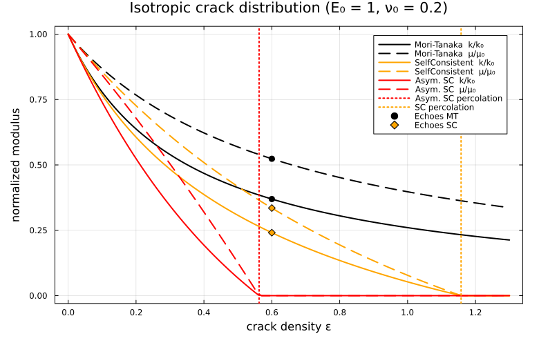

The numerics confirm both: to six decimals, and for the stiffness form — later by a factor , so very nearly twice the crack density.

That gap is what makes the chosen   a revealing test point: it sits between the two thresholds, so AsymmetricSelfConsistent returns zero there while SelfConsistent still returns the finite medium that Echoes reports. Neither is wrong — they are two different definitions of "embed each phase in the effective medium", and which one to trust is a modeling decision, not a numerical one.

Parallel cracks

One orientation, so the effective tensor is transversely isotropic about the crack normal. Reading it back needs one convention to be clear, and it is the one that trips people up:

C_par = homogenize(rve_parallel(ε), MoriTanaka(), :C)
typeof(C_par)

TensND.TensRotated{4, 3, Float64, Tensors.SymmetricTensor{4, 3, Float64, 36}}

The result is a TensRotated: it carries its own frame. TensND.KM then returns the components in that frame — the crack frame — not in the global one. Both are useful, and they are different matrices:

C_local = TensND.KM(C_par)                              # crack frame
C_global = TensND.KM(TensND.components_canon(C_par))    # global frame
round.(C_local; digits = 6)

6×6 Matrix{Float64}:
 1.0574    0.224068  0.062941  0.0       0.0       0.0
 0.224068  1.0574    0.062941  0.0       0.0       0.0
 0.062941  0.062941  0.251762  0.0       0.0       0.0
 0.0       0.0       0.0       0.344037  0.0       0.0
 0.0       0.0       0.0       0.0       0.344037  0.0
 0.0       0.0       0.0       0.0       0.0       0.833333

In the crack frame the transverse isotropy is plain: the 3-axis is the normal, the block is the crack plane, and the last two diagonal entries are the out-of-plane and in-plane shears.

round.(C_global; digits = 6)

6×6 Matrix{Float64}:
  0.902533   0.166717   0.154314  -0.060764  -0.208074  -0.180198
  0.166717   0.639222   0.175933  -0.284582   0.008689  -0.142291
  0.154314   0.175933   0.53078   -0.246676  -0.142418   0.026478
 -0.060764  -0.284582  -0.246676   0.590902   0.00128   -0.029472
 -0.208074   0.008689  -0.142418   0.00128    0.589424  -0.158264
 -0.180198  -0.142291   0.026478  -0.029472  -0.158264   0.635111

The global matrix is full, and it is the one to compare against another code that knows nothing of the crack frame. The five Walpole coefficients — the reporting form Echoes prints as Param(size=5) — come straight from the local matrix:

walpole = TensND.ti_params_from_KM(C_local)
round.(collect(walpole); digits = 6)

5-element Vector{Float64}:
 0.251762
 1.28147
 0.089011
 0.833333
 0.344037

Against Echoes 1.0, same problem, same density:

echoes_parallel = [0.251762, 1.28147, 0.0890113, 0.833333, 0.344036]
@printf "max |Δ| on the five Walpole coefficients : %.2e\n" maximum(
    abs.(collect(walpole) .- echoes_parallel)
)

max |Δ| on the five Walpole coefficients : 6.97e-07

The fourth coefficient is exactly  : the shear that acts in the crack plane is not relaxed by an opening at all, whatever the density. That is a useful check that the orientation survived the whole pipeline.

One scheme is unavailable here

SelfConsistent on a single-orientation crack phase raises a SingularException: its strain-concentration tensor degenerates when the inclusion has no volume and no orientation average smooths it. Use AsymmetricSelfConsistent, as the cracks manual prescribes — bearing in mind, from the previous section, that it is a different fixed point from Echoes' SC.

try
    homogenize(rve_parallel(ε), SC, :C)
catch err
    println("SelfConsistent : ", first(sprint(showerror, err), 60))
end

C_par_asc = homogenize(rve_parallel(ε), ASC, :C)
round.(collect(TensND.ti_params_from_KM(TensND.KM(C_par_asc))); digits = 6)

5-element Vector{Float64}:
 0.014504
 1.251813
 0.005128
 0.833333
 0.192086

Isotropic against parallel, at equal density

The last comparison is the point of the whole page: same cracks, same , and a Young's modulus that depends on the direction it is measured in only in the second case.

function young_along(C, d)
    # Uniaxial stress along the unit vector `d`; E = σ / ε_dd.
    S = inv(Array(TensND.components_canon(C)) |> A -> TensND.KM(TensND.Tens(A)))
    e = [d[1]^2, d[2]^2, d[3]^2, √2 * d[2] * d[3], √2 * d[1] * d[3], √2 * d[1] * d[2]]
    return 1 / (e' * S * e)
end

C_iso = homogenize(rve_isotropic(ε), MoriTanaka(), :C)
angles = range(0, π; length = 181)
# Directions swept in the plane containing the crack normal.
t̂ = normalize(cross(collect(normal), [0.0, 0.0, 1.0]))
dirs = [cos(a) .* collect(normal) .+ sin(a) .* t̂ for a in angles]

p_dir = plot(;
    proj = :polar, size = (620, 560), legend = :bottomleft,
    title = "Young's modulus in the plane of the crack normal, ε = $ε"
)
plot!(p_dir, angles, [young_along(C_iso, d) for d in dirs];
    lw = 2.5, color = :black, label = "isotropic distribution")
plot!(p_dir, angles, [young_along(C_par, d) for d in dirs];
    lw = 2.5, color = :red, label = "parallel cracks")
p_dir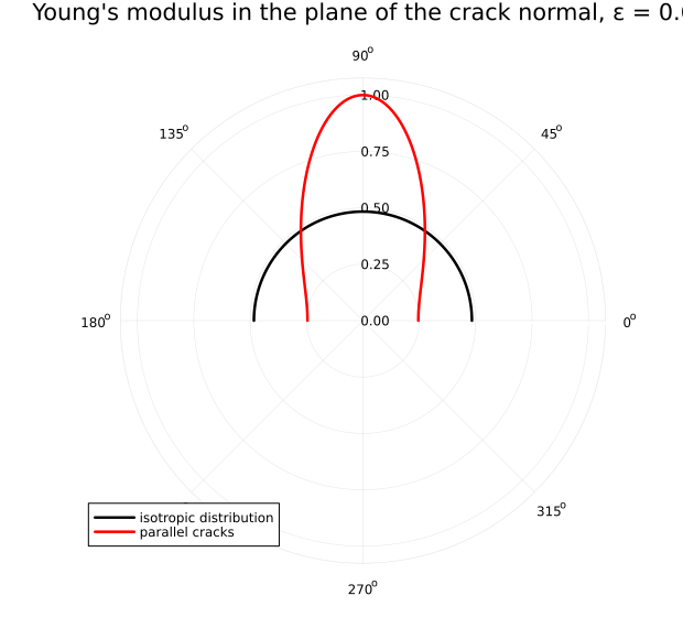

At   the direction is the crack normal, where the parallel population is at its softest; at   it lies in the crack plane, where opening contributes nothing and the modulus is close to the intact one. The isotropic distribution flattens that contrast into a single number — the same amount of cracking, spread over every orientation.

---

This page was generated using Literate.jl.