
Viscoelastic composites
Every scheme seen so far takes an elastic stiffness tensor and returns an elastic stiffness tensor. The correspondence principle extends this, almost for free, to linear viscoelasticity: replace real moduli by their complex, frequency-dependent counterparts, and the exact same schemes carry through.
Complex moduli in the frequency domain
A Maxwell-type viscoelastic shear modulus has the classical form
real (elastic) at zener_maxwell — so it is written below with iso_rheology rather than by hand. Building an RVE with the resulting complex-valued stiffness and calling homogenize exactly as before propagates that complex modulus through the homogenization algebra — every scheme is Complex{Float64}-safe:
using MeanFieldHomogenization
using TensND
using LinearAlgebra
using Plots
gr()  # headless backend; GKSwstype is set to "100" in make.jl

## One model per phase: an elastic bulk channel, a standard-solid shear one.
PHASE_M = iso_rheology(Spring(30.0), zener_maxwell(10.0, 5.0, 1.0))
PHASE_I = iso_rheology(Spring(80.0), zener_maxwell(30.0, 15.0, 1.0))

const f_inc = 0.3
ωs = exp10.(range(-2, 2; length = 40))

function C_eff_at(ω, scheme)
    p = im * ω
    r = RVE()
    add_phase!(r, :M, Ellipsoid(1.0), Dict(:C => carson_relaxation(PHASE_M, p)); fraction = :rest)
    add_phase!(r, :I, Ellipsoid(1.0), Dict(:C => carson_relaxation(PHASE_I, p)); fraction = f_inc)
    _, μ = k_mu(homogenize(r, scheme, :C))
    return μ
end

y_mt = [C_eff_at(ω, MoriTanaka()) for ω in ωs]
y_sc = [C_eff_at(ω, SelfConsistent(; abstol = 1.0e-10, maxiters = 200)) for ω in ωs]

plt = plot(;
    xlabel = "ω", ylabel = "μ_eff", xscale = :log10,
    legend = :topleft, framestyle = :box, size = (760, 480),
)
plot!(plt, ωs, real.(y_mt); label = "storage — MT", color = :blue, lw = 2)
plot!(plt, ωs, imag.(y_mt); label = "loss — MT", color = :blue, lw = 2, ls = :dash)
plot!(plt, ωs, real.(y_sc); label = "storage — SC", color = :red, lw = 2)
plot!(plt, ωs, imag.(y_sc); label = "loss — SC", color = :red, lw = 2, ls = :dash)
plt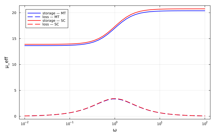
The real part (storage modulus) rises from the low-frequency to the high-frequency elastic limit, and the imaginary part (loss modulus) peaks in between, at the frequency where the microstructure's relaxation time and the loading period coincide — the qualitative signature of any viscoelastic composite, MT and SC differing only in how strongly the inclusion phase influences the peak's height and position through interaction.
Nothing to declare on the RVE
Complex-valued homogenization needs no element type on the RVE: the moduli carry the complex part, the volume fraction stays real, and the two are promoted where they meet. RVE() is enough — the RVE{ComplexF64}() / RVE(; T = ComplexF64) forms only declare a floor for the amounts and give the same numbers.
One gap, in the complex plane only: SelfConsistent(algorithm = NewtonDefault()) builds its Jacobian with ForwardDiff, which cannot carry a Dual over a complex scalar. The default Anderson solver is the complex-capable path — and so is the Laplace-Carson route with GaverStehfest, whose Carson variables are all real, so the Newton solver never meets a complex number in the first place.
A first taste of time-domain ageing viscoelasticity
The frequency-domain view above assumes properties that do not evolve with the material's age. For ageing viscoelasticity — a material whose relaxation spectrum itself changes with time, as in curing cement paste — MeanFieldHomogenization provides a full time-domain (ALV) pipeline built on discretized Volterra operators. A ViscoLaw wraps a two-argument relaxation kernel R(t, t'), and homogenize_alv takes the place of homogenize:
function R_iso(t, tp)
    α = 3 * (3.0 + 2.0 * exp(-(t - tp) / 1.0))
    β = 2 * (1.0 + 1.0 * exp(-(t - tp) / 0.5))
    return TensISO{3}(α, β)
end
law_M = ViscoLaw(R_iso, :relaxation)

rve = RVE()
add_phase!(rve, :M, Ellipsoid(1.0), Dict(:C => law_M); fraction = :rest)
add_phase!(rve, :I, Ellipsoid(1.0), Dict(:C => heaviside_law(iso_stiffness(60.0, 20.0))); fraction = 0.2)

times = collect(range(0.0, 5.0; length = 20))
C_eff = homogenize_alv(rve, MoriTanaka(), :C; times = times)
size(C_eff)
(120, 120)The result is a discretized Volterra operator (a dense block matrix, here 40×40 since each of the 20 time steps carries a 2×2 iso block), not a single tensor — reading effective moduli back out of it, handling cracks in ALV, and differentiating through the whole pipeline are covered in full in the Viscoelasticity manual.
…and back to the time domain
The frequency route above stops at
cell(p) = begin
    r = RVE()
    add_phase!(r, :M, Ellipsoid(1.0), Dict(:C => carson_relaxation(PHASE_M, p)); fraction = :rest)
    add_phase!(r, :I, Ellipsoid(1.0), Dict(:C => carson_relaxation(PHASE_I, p)); fraction = f_inc)
    r
end

μ_t = [k_mu(C)[2] for C in homogenize_lc(cell, MoriTanaka(), :C; times = [0.05, 0.5, 5.0])]
3-element Vector{Float64}:
20.05491594680336
17.736574537704033
13.691043599234542That is homogenize_lc, and it is the subject of three further tutorials: the model catalog, the exact Kelvin ⇄ Maxwell conversion, and how to choose an inversion algorithm. The three-route comparison then checks this route, the frequency one and the ageing one against each other on the same composite.
The next two tutorials return to elastic problems and build up to differentiating homogenize itself.