A first homogenization

Every MeanFieldHomogenization computation starts from the same three ingredients: a representative volume element (RVE) describing the phases, their geometry, and a scheme that turns the RVE into a single effective property. This page builds the simplest possible RVE — a matrix with one spherical inclusion phase — and computes its effective stiffness two different ways.

Building an RVE

using MeanFieldHomogenization
using TensND
using LinearAlgebra
using Plots
gr()  # headless backend; GKSwstype is set to "100" in make.jl

rve = RVE()
add_phase!(rve, :M, Ellipsoid(1.0), Dict(:C => iso_stiffness(30.0, 10.0)); fraction = :rest)
add_phase!(rve, :I, Ellipsoid(1.0), Dict(:C => iso_stiffness(60.0, 20.0)); fraction = 0.2)
rve

RVE{Float64} with 2 phase(s)
  phase :M   f = 0.8  (rest)
  phase :I   f = 0.2
  closure : ComplementFraction(:warn)
  distribution_shape : none declared (Maxwell / PCW will ask for one)

RVE() creates an empty container; add_phase! then attaches a geometry (here Ellipsoid(1.0), a unit sphere), a property dictionary and an amount to each phase. fraction = 0.2 means 20 % of the RVE by volume; fraction = :rest means "whatever the others leave", here 80 %.

Note that nothing so far says which phase is a matrix — that is the scheme's to decide, and MoriTanaka() below takes the :rest phase because it is the only candidate. See Who is the matrix?.

A storage convention worth knowing

iso_stiffness(k, mu) builds the isotropic stiffness tensor from the physical bulk and shear moduli and . Internally TensND stores an isotropic 4th-order tensor as the raw pair — so TensISO{3}(a, b) interprets its two arguments as that pair directly, not as :

C1 = iso_stiffness(30.0, 10.0)      # from physical (k, μ) = (30, 10)
C2 = TensISO{3}(3 * 30.0, 2 * 10.0)  # same tensor, built from the raw pair
C1 == C2

true

Recover the physical moduli from either with k_mu:

k_mu(C1)

(30.0, 10.0)

To avoid this trap, every example in these tutorials builds isotropic stiffnesses with iso_stiffness(k, mu) and reads results back with k_mu.

The dilute estimate

The simplest scheme, Dilute, assumes each inclusion sits in an infinite matrix, ignoring every other inclusion around it. The effective stiffness is a sum of independent contributions:

where is the Hill polarization tensor of inclusion in the matrix (hill_tensor) and is its dilute strain-localization tensor: the linear map from the macroscopic strain to the strain inside inclusion . This is exact only in the dilute limit   — at finite volume fraction, inclusions interact and the estimate drifts.

Mori–Tanaka: accounting for interaction

MoriTanaka corrects for this by localizing not on the macroscopic strain, but on the average strain in the matrix:

Both schemes are called the same way — only the scheme argument to homogenize changes:

k_dil, _ = k_mu(homogenize(rve, Dilute(), :C))
k_mt, _ = k_mu(homogenize(rve, MoriTanaka(), :C))
(k_dil, k_mt)

(33.54545454545455, 33.86138613861386)

Comparing the two across volume fraction

function build(f)
    r = RVE()
    add_phase!(r, :M, Ellipsoid(1.0), Dict(:C => iso_stiffness(30.0, 10.0)); fraction = :rest)
    add_phase!(r, :I, Ellipsoid(1.0), Dict(:C => iso_stiffness(60.0, 20.0)); fraction = f)
    return r
end

fs = exp10.(range(-4, log10(0.6); length = 30))
k_dil = [k_mu(homogenize(build(f), Dilute(), :C))[1] for f in fs]
k_mt = [k_mu(homogenize(build(f), MoriTanaka(), :C))[1] for f in fs]

plt = plot(;
    xlabel = "inclusion volume fraction f", ylabel = "k_eff",
    xscale = :log10, legend = :topleft, framestyle = :box, size = (760, 480),
)
plot!(plt, fs, k_dil; label = "Dilute", lw = 2)
plot!(plt, fs, k_mt; label = "MoriTanaka", lw = 2)
hline!(plt, [k_dil[1]]; label = "matrix", lw = 1, color = :gray, ls = :dash)
plt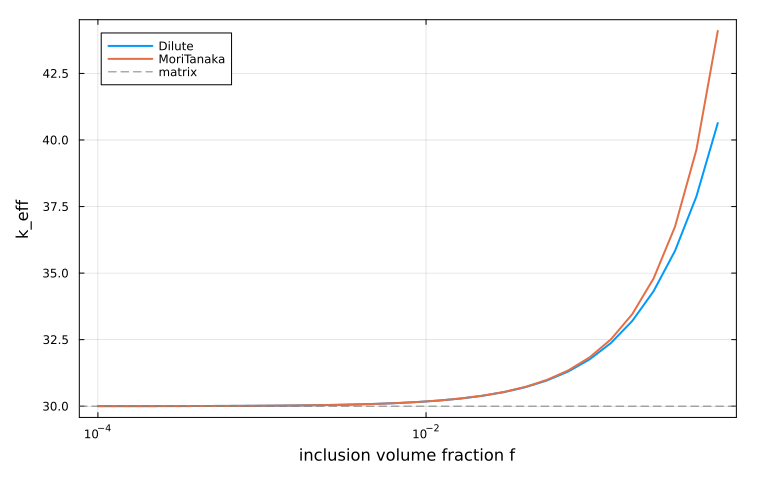

The two curves coincide as   — both schemes agree in the dilute limit, as they must — and diverge as grows: at finite volume fraction the inclusions interact, and Mori–Tanaka, which accounts for that, departs from the naive dilute sum.