
Generalized Kelvin ⇄ generalized Maxwell
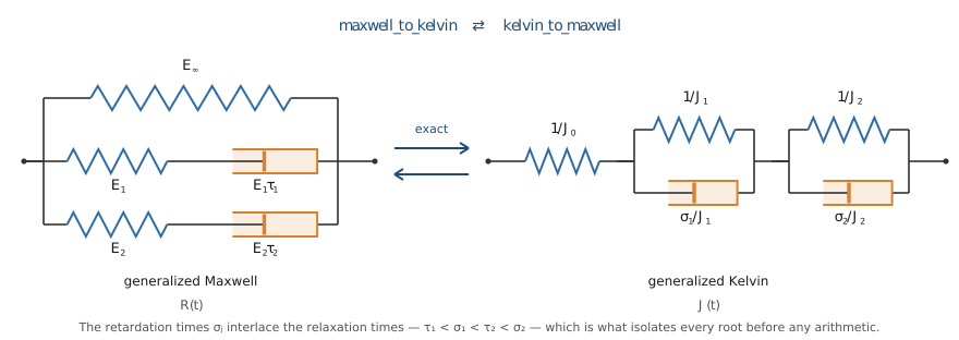
A viscoelastic solid can be written two ways. Springs and dashpots in series branches parallel to an equilibrium spring give a generalized Maxwell chain, described by a relaxation function; springs and dashpots in parallel cells stacked in series give a generalized Kelvin chain, described by a creep function:
They describe the same material, so one must be computable from the other. In the time domain that is a deconvolution; in the Laplace-Carson domain it is a single line,
and since both transforms are rational in p, passing from one chain to the other is nothing but a partial-fraction decomposition.
This page shows what maxwell_to_kelvin and kelvin_to_maxwell do, why the structure of the problem makes them unconditionally robust, and checks them against two independent closed forms.
using MeanFieldHomogenization
using Printf
using Plots
gr() # headless backend; GKSwstype is set to "100" before Literate runsPlots.GRBackend()§1 One conversion, and what it produces
Take the two-branch Maxwell chain of the ECHOES reference Kelvin2Maxwell.py: an equilibrium spring E_∞ = 8 and branches (3, τ=12) and (17, τ=23).
maxwell = PronyRelaxation(8.0, [3.0, 17.0], [12.0, 23.0])
kelvin = maxwell_to_kelvin(maxwell)

@printf "Maxwell : E_∞ = %.4f,  E = %s,  τ = %s\n" maxwell.E_inf string(maxwell.E) string(maxwell.tau)
@printf "Kelvin  : J_0 = %.6f,  J = %s,  τ = %s,  φ = %.3g\n" kelvin.J_0 string(round.(kelvin.J; sigdigits = 6)) string(round.(kelvin.tau; sigdigits = 6)) kelvin.phi
Maxwell : E_∞ = 8.0000, E = [3.0, 17.0], τ = [12.0, 23.0]
Kelvin : J_0 = 0.035714, J = [0.00123891, 0.0880468], τ = [12.7783, 75.5967], φ = 0The conversion is exact, not fitted. The product of the two transforms is 1 to machine precision, everywhere on the positive real axis and off it:
for p in (1.0e-6, 1.0e-3, 0.037, 1.0, 37.0, 1.0e4)
    @printf "  p = %-9.3g   J*(p) R*(p) - 1 = %+.3e\n" p (carson_creep(kelvin, p) * carson_relaxation(maxwell, p) - 1)
end
p = 1e-06 J*(p) R*(p) - 1 = +0.000e+00
p = 0.001 J*(p) R*(p) - 1 = +2.220e-16
p = 0.037 J*(p) R*(p) - 1 = +0.000e+00
p = 1 J*(p) R*(p) - 1 = -1.110e-16
p = 37 J*(p) R*(p) - 1 = +0.000e+00
p = 1e+04 J*(p) R*(p) - 1 = +0.000e+00§2 Why it cannot fail: interlacing
The reference implementation expands R^{*}(p)\prod_i(1+p\tau_i) into a polynomial and hands its roots to a symbolic root-finder. That is exact on paper and badly conditioned in practice — real relaxation spectra have dozens of branches spread over six to ten decades, and a polynomial of that degree cannot be formed in floating point without losing its roots.
There is a much better structure available. Substituting
a function that is strictly increasing between consecutive poles and sweeps from -∞ to +∞ across every gap. Its zeros are the retardation times we are looking for, and they therefore interlace the relaxation times: exactly one in each (τ_j, τ_{j+1}), and one beyond the last pole when the material is a solid. Each unknown is isolated before any arithmetic happens, so bisection in log σ finds it whatever the number of branches or their spread.
# A spectrum with well-separated times, so the alternation is visible.
demo = PronyRelaxation(1.0, [2.0, 3.0, 1.5], [1.0, 10.0, 100.0])
demo_k = maxwell_to_kelvin(demo)

σ = exp10.(range(-0.5, 4.0; length = 4000))
Φ_clipped = clamp.([carson_relaxation(demo, -1 / s) for s in σ], -8, 8)

p_interlace = plot(
    σ, Φ_clipped;
    xscale = :log10, lw = 2, color = :black, label = "Φ(σ) = R*(-1/σ)",
    xlabel = "σ  (retardation-time variable)", ylabel = "Φ(σ)",
    ylims = (-8, 8), legend = :bottomright,
    title = "Zeros of R* interlace its poles"
)
hline!(p_interlace, [0.0]; color = :grey, ls = :dot, label = "")
vline!(p_interlace, demo.tau; color = :crimson, ls = :dash, lw = 2, label = "poles τ_j (Maxwell)")
vline!(p_interlace, demo_k.tau; color = :royalblue, lw = 2, label = "zeros σ_j (Kelvin)")
scatter!(p_interlace, demo_k.tau, zeros(length(demo_k.tau)); color = :royalblue, ms = 6, label = "")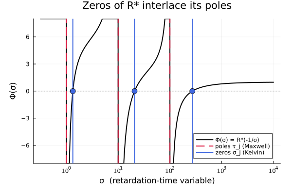
Read the alternation straight off the axis: between each pair of red poles there is exactly one blue zero, and one more beyond the last pole because E_∞ > 0. For a fluid that last zero recedes to infinity, and that is the series dashpot of the Kelvin form.
@printf "poles τ_j : %s\n" string(demo.tau)
@printf "zeros σ_j : %s\n" string(round.(demo_k.tau; sigdigits = 6))
@printf "interlaced: %s\n" all(demo.tau[i] < demo_k.tau[i] < demo.tau[i + 1] for i in 1:2)
poles τ_j : [1.0, 10.0, 100.0]
zeros σ_j : [1.33432, 20.7473, 270.918]
interlaced: true§3 The two functions of time
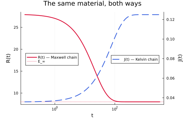
With both chains in hand, R(t) and J(t) are closed-form sums — and their product is not one, because in the time domain the reciprocal relation is a convolution. What must hold instead is the Volterra identity
ts = exp10.(range(-1, 3.5; length = 300))
p_time = plot(
    ts, [relaxation(maxwell, t) for t in ts];
    xscale = :log10, lw = 2.5, color = :crimson, label = "R(t) — Maxwell chain",
    xlabel = "t", ylabel = "R(t)", legend = :left,
    title = "The same material, both ways"
)
hline!(p_time, [maxwell.E_inf]; color = :crimson, ls = :dot, label = "E_∞")
p_time2 = twinx(p_time)
plot!(
    p_time2, ts, [creep(kelvin, t) for t in ts];
    xscale = :log10, lw = 2.5, color = :royalblue, ls = :dash,
    label = "J(t) — Kelvin chain", ylabel = "J(t)", legend = :right
)
§4 Round trip, and the regime the symbolic route cannot reach
Converting back must return the input exactly. Below, a chain with an increasing number of branches log-spaced over six decades is sent through maxwell_to_kelvin and back, and the worst relative error on any recovered (E_i, τ_i) is plotted. This is the regime — a dozen branches and more — where forming the polynomial loses its roots entirely.
function roundtrip_error(n)
    τ = exp10.(range(-3, 3; length = n))
    m = PronyRelaxation(2.0, fill(1.0, n), τ)
    back = kelvin_to_maxwell(maxwell_to_kelvin(m))
    return max(
        maximum(abs.(back.E .- m.E) ./ m.E),
        maximum(abs.(back.tau .- m.tau) ./ m.tau),
        abs(back.E_inf - m.E_inf) / m.E_inf
    )
end

branch_counts = 2:2:20
errors = [roundtrip_error(n) for n in branch_counts]

p_roundtrip = plot(
    branch_counts, max.(errors, 1.0e-17);
    yscale = :log10, lw = 2.5, marker = :circle, color = :seagreen, label = "",
    xlabel = "number of branches, spread over 6 decades",
    ylabel = "worst relative round-trip error",
    title = "Kelvin → Maxwell → Kelvin", ylims = (1.0e-17, 1.0e-10)
)
hline!(p_roundtrip, [eps(Float64)]; color = :grey, ls = :dash, label = "eps(Float64)")

@printf "worst round-trip error at 20 branches : %.2e\n" errors[end]
worst round-trip error at 20 branches : 1.11e-15§5 Two independent closed forms as oracles
The Zener relations
For a single branch the conversion has a classical closed form, printed as a check by the ECHOES script itself. With E_∞ the equilibrium spring and (E_1, τ_1) the Maxwell branch, and η = E_1 τ_1,
and the retardation time must come out equal to both
E0, E1, τ1 = 8.0, 3.0, 12.0
z = maxwell_to_kelvin(zener_maxwell(E0, E1, τ1))
η = E1 * τ1
J0_ref = 1 / (E0 + E1)
J1_ref = 1 / E0 - J0_ref
η1 = η * ((E0 + E1) / E1)^2

@printf "J_0    : computed %.12f   reference %.12f\n" z.J_0 J0_ref
@printf "J_1    : computed %.12f   reference %.12f\n" z.J[1] J1_ref
@printf "τ^K    : computed %.12f   η₁J₁ = %.12f   τ₁(E₀+E₁)/E₀ = %.12f\n" z.tau[1] (η1 * J1_ref) (τ1 * (E0 + E1) / E0)
J_0 : computed 0.090909090909 reference 0.090909090909
J_1 : computed 0.034090909091 reference 0.034090909091
τ^K : computed 16.500000000000 η₁J₁ = 16.500000000000 τ₁(E₀+E₁)/E₀ = 16.500000000000Burgers, and the fluid branch
The Burgers model is a Maxwell unit in series with a Kelvin cell — a fluid, whose creep compliance grows linearly for ever. Its Kelvin form has one branch; its Maxwell form must therefore have two, with no equilibrium spring, because the rational transform has one more pole than the Kelvin chain has branches.
Its relaxation function was derived independently in closed form (a cosh/sinh expression, transcribed here from the ECHOES reference fluage_echoes_ijss2013_jsanahuja_relaxBurgers.py), which makes it the ideal oracle for the fluid path: degenerate-branch detection, the unbounded outermost bracket and both residue signs are all exercised at once.
ks, ηs, kp, ηp = 1.0, 3.0, 2.0, 6.0
b = burgers(ks, ηs, kp, ηp)
b_maxwell = kelvin_to_maxwell(b)

@printf "Burgers is a fluid : %s\n" is_fluid(b)
@printf "  Kelvin form  : 1 branch + a series dashpot (φ = %.4f)\n" b.phi
@printf "  Maxwell form : %d branches, E_∞ = %.3e, E = %s, τ = %s\n" length(b_maxwell) b_maxwell.E_inf string(round.(b_maxwell.E; sigdigits = 6)) string(round.(b_maxwell.tau; sigdigits = 6))

function burgers_relaxation_closed_form(t)
    d = sqrt(
        ηp^2 * ks^2 - 2ηp * ηs * ks * kp + 2ηp * ηs * ks^2 +
            ηs^2 * kp^2 + 2ηs^2 * kp * ks + ηs^2 * ks^2
    )
    return exp(-0.5t * kp / ηp - 0.5t * ks / ηp - 0.5t * ks / ηs) * (
        ks * cosh(0.5t * d / (ηp * ηs)) +
            sinh(0.5t * d / (ηp * ηs)) * (-ηp * ks + ηs * kp - ks * ηs) * ks / d
    )
end

tb = range(0.0, 25.0; length = 300)
R_converted = [relaxation(b_maxwell, t) for t in tb]
R_closed = [burgers_relaxation_closed_form(t) for t in tb]

p_burgers = plot(
    tb, R_closed;
    lw = 4, color = :lightgrey, label = "closed form (independent derivation)",
    xlabel = "t", ylabel = "R(t)", title = "Burgers relaxation — fluid path"
)
plot!(p_burgers, tb, R_converted; lw = 2, color = :darkorange, ls = :dash, label = "kelvin_to_maxwell")

p_burgers_err = plot(
    tb[2:end], max.(abs.(R_converted[2:end] .- R_closed[2:end]), 1.0e-18);
    yscale = :log10, lw = 2, color = :darkorange, label = "",
    xlabel = "t", ylabel = "|difference|  (floored at 1e-18)",
    title = "…agreeing to machine precision"
)

@printf "worst |R_converted - R_closed| over t ∈ [0, 25] : %.2e\n" maximum(abs.(R_converted .- R_closed))
Burgers is a fluid : true
Kelvin form : 1 branch + a series dashpot (φ = 0.3333)
Maxwell form : 2 branches, E_∞ = 0.000e+00, E = [0.666667, 0.333333], τ = [1.5, 6.0]
worst |R_converted - R_closed| over t ∈ [0, 25] : 1.11e-16§6 Fitting a chain to something that is not one
The conversion needs a Prony chain to start from. When the material is given as an arbitrary transform instead — a fractional model, or a homogenized C*(p) — prony_fit_relaxation fits one by collocation, and everything above becomes available: a closed-form time function, an exact dual chain, and a ViscoLaw for the ageing pipeline.
fz = FractionalZener(2.0, 10.0, 1.0, 0.6)
τ_trial = exp10.(range(-2, 2; length = 14))
fitted = prony_fit_relaxation(p -> carson_relaxation(fz, p), τ_trial)

ω = exp10.(range(-4, 4; length = 200))
p_fit = plot(
    ω, [abs(complex_modulus(fz, w)) for w in ω];
    xscale = :log10, yscale = :log10, lw = 3, color = :black,
    label = "FractionalZener (α = 0.6)",
    xlabel = "ω", ylabel = "|E*(ω)|", legend = :bottomright,
    title = "A 14-branch Prony fit of a fractional model"
)
plot!(p_fit, ω, [abs(complex_modulus(fitted, w)) for w in ω]; lw = 2, ls = :dash, color = :purple, label = "Prony fit, $(length(fitted)) branches")

# Lawson-Hanson NNLS is an active-set method, so it returns a *sparse*
# spectrum: here 7 of the 14 trial times carry weight and the rest are
# exactly zero.  Only the active ones are worth drawing.
active = findall(>(0), fitted.E)
p_fit_spectrum = scatter(
    fitted.tau[active], fitted.E[active];
    xscale = :log10, color = :purple, ms = 6, label = "active branches",
    xlabel = "τ_i", ylabel = "E_i",
    title = "the fitted discrete spectrum", legend = :topright
)
for i in active
    plot!(p_fit_spectrum, [fitted.tau[i], fitted.tau[i]], [0.0, fitted.E[i]]; color = :purple, lw = 2, label = "")
end
hline!(p_fit_spectrum, [0.0]; color = :grey, ls = :dot, label = "")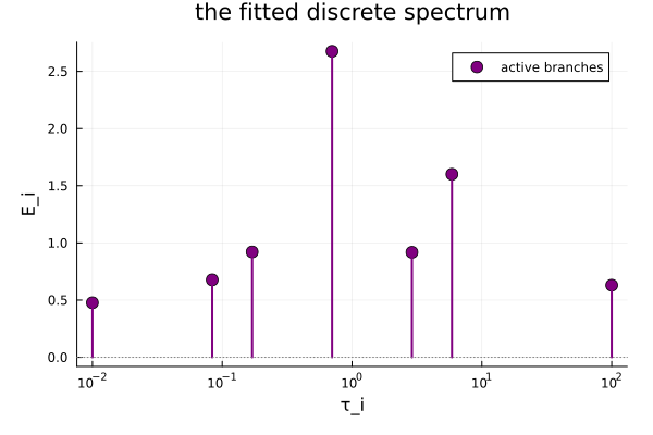
The fit is non-negative by default. That is not only a matter of physical admissibility — a non-negative spectrum is what makes the fitted function completely monotone, hence passive — it also happens to fit better here: the unconstrained least-squares solution puts seven of the fourteen moduli below zero and is three times worse on the master curve.
rel_err(f) = maximum(abs(abs(complex_modulus(f, w)) - abs(complex_modulus(fz, w))) / abs(complex_modulus(fz, w)) for w in ω)
unconstrained = prony_fit_relaxation(p -> carson_relaxation(fz, p), τ_trial; nonneg = false)

@printf "non-negative fit : %d/%d active branches, worst |E*| error %.1f %%\n" count(>(0), fitted.E) length(fitted) (100 * rel_err(fitted))
@printf "unconstrained    : %d negative moduli,   worst |E*| error %.1f %%\n" count(<(0), unconstrained.E) (100 * rel_err(unconstrained))
@printf "loss factor stays ≥ 0 : %s\n" all(loss_factor(fitted, w) ≥ -1.0e-12 for w in ω)

p_full = plot(
    p_interlace, p_roundtrip, p_burgers, p_burgers_err, p_fit, p_fit_spectrum;
    layout = (3, 2), size = (1300, 1300),
    left_margin = 6Plots.mm, bottom_margin = 6Plots.mm
)
p_full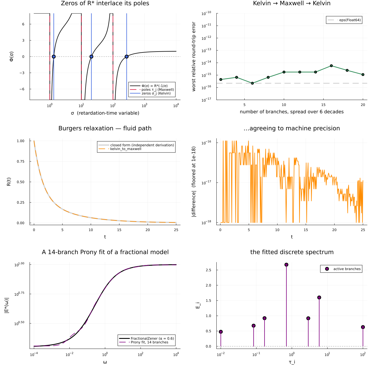
This page was generated using Literate.jl.