
The cluster model on cubic arrays
The cluster model of [1] solves for the mean strain of every inclusion, accounting for the pairwise interaction with each neighbor inside a cluster of radius R_c. Unlike the one-site schemes it therefore sees where the inclusions are, which is why it acts on a ParticleAssembly rather than on an RVE.
This page reproduces the reference results of their §4 on simple-cubic arrays of stiff spheres: the convergence in cluster radius (their Fig. 3), the comparison with the other schemes of the package (their Fig. 5) and with Mori-Tanaka in particular (their Fig. 6).
The scheme rests on the two-inclusion interaction tensor
whose self counterpart is
using MeanFieldHomogenization
using TensND
using Printf
using Plots
gr()

default(; left_margin = 5Plots.mm, bottom_margin = 5Plots.mm)
Matrix: k = 1, μ = 0.4 (hence ν = 0.3, the value used throughout the paper). "Rigid" spheres are four orders of magnitude stiffer, which is numerically indistinguishable from the rigid limit at these contrasts.
k_m, μ_m = 1.0, 0.4
C_m = TensISO{3}(3k_m, 2μ_m)
C_rigid = TensISO{3}(3 * 1.0e4, 2 * 1.0e4)
C_void = TensISO{3}(3 * 1.0e-9, 2 * 1.0e-9)

μ_of(C) = get_array(C)[1, 2, 1, 2]
κ_of(C) = (A = get_array(C); sum(A[i, i, j, j] for i in 1:3, j in 1:3) / 9)
κ_of (generic function with 1 method)The one-site schemes read the same assembly: RVE(asm) forgets the positions and keeps the derived fractions, so no parallel cell has to be built by hand for the comparisons below — and none can silently drift out of step with the assembly it is meant to mirror.
§1 Convergence in the cluster radius
Their Fig. 3. Below one period the cluster contains no neighbor at all and the scheme degenerates exactly onto Mori-Tanaka — the identity proved in their Appendix C. Beyond R_c ≈ 2 periods the estimate is flat; the residual wobble is the discrete shell structure of a spherical cutoff, visible in their own figure too.
cutoffs = 0.0:0.25:5.0
conv = Dict{Float64, Vector{Float64}}()
for f in (0.2, 0.5)
    conv[f] = [
        μ_of(
            homogenize(
                cubic_lattice(
                    :sc, Dict(:C => C_m), Dict(:C => C_rigid);
                    fraction = f, cutoff = c
                ), ClusterModel(), :C
            )
        ) / μ_m for c in cutoffs
    ]
end

for f in (0.2, 0.5)
    @printf "f = %.1f :  Mori-Tanaka %.4f   cluster(R_c=0) %.4f   cluster(R_c=3) %.4f\n" f (μ_of(homogenize(cubic_lattice(:sc, Dict(:C => C_m), Dict(:C => C_rigid); fraction = f), MoriTanaka(), :C)) / μ_m) conv[f][1] conv[f][13]
end

p1 = plot(;
    xlabel = "R_c / L", ylabel = "μ_eff / μ_m",
    title = "Convergence in cluster radius (SC, rigid spheres)",
    legend = :right
)
for f in (0.2, 0.5)
    plot!(p1, cutoffs, conv[f]; marker = :circle, ms = 3, label = "cluster, f = $f")
    hline!(
        p1, [μ_of(homogenize(cubic_lattice(:sc, Dict(:C => C_m), Dict(:C => C_rigid); fraction = f), MoriTanaka(), :C)) / μ_m];
        ls = :dash, label = "Mori-Tanaka, f = $f"
    )
end
p1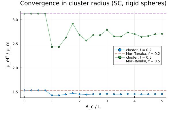
§2 Against the other schemes of the package
Their Fig. 5 and Fig. 6. The one-site self-consistent scheme is unsuited to a matrix-inclusion morphology — it does not see the connectivity of the matrix — while the three-phase and differential schemes, which do, sit much closer to the cluster estimate. Mori-Tanaka overestimates the shear modulus here: for a simple-cubic (i.e. non-isotropic) distribution of stiff spheres it is not a bound.
fracs = 0.05:0.05:0.45
cluster = Float64[]
mt = Float64[]
sc = Float64[]
diff_ = Float64[]
for f in fracs
    asm = cubic_lattice(
        :sc, Dict(:C => C_m), Dict(:C => C_rigid); fraction = f, cutoff = 3.0
    )
    push!(cluster, μ_of(homogenize(asm, ClusterModel(), :C)) / μ_m)
    push!(mt, μ_of(homogenize(asm, MoriTanaka(), :C)) / μ_m)
    push!(sc, μ_of(homogenize(asm, SelfConsistent(), :C)) / μ_m)
    push!(diff_, μ_of(homogenize(asm, DifferentialScheme(; nsteps = 200), :C)) / μ_m)
end

p2 = plot(
    fracs, cluster;
    marker = :circle, ms = 3, label = "cluster (R_c = 3L)",
    xlabel = "f", ylabel = "μ_eff / μ_m",
    title = "Simple-cubic array of rigid spheres", legend = :topleft
)
plot!(p2, fracs, mt; marker = :square, ms = 3, ls = :dash, label = "Mori-Tanaka")
plot!(p2, fracs, sc; marker = :diamond, ms = 3, ls = :dot, label = "self-consistent")
plot!(p2, fracs, diff_; marker = :utriangle, ms = 3, ls = :dashdot, label = "differential")
p2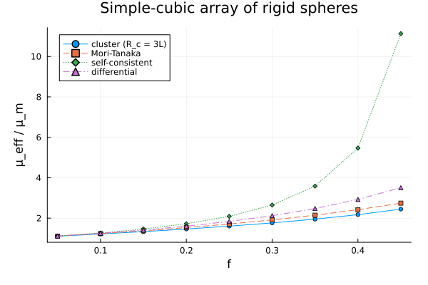
§3 What the cluster changes, and what it cannot
The interaction tensor has a strictly vanishing isotropic part, so summing it over a cluster cannot alter the spherical part of the problem. The effective bulk modulus of a cubic array is therefore exactly the Mori-Tanaka one, at every volume fraction — only the shear response sees the arrangement.
println("\n  f      κ_cluster / κ_MT      μ_cluster / μ_MT")
for f in (0.1, 0.2, 0.3, 0.4)
    asm = cubic_lattice(:sc, Dict(:C => C_m), Dict(:C => C_rigid); fraction = f, cutoff = 3.0)
    Ccl = homogenize(asm, ClusterModel(), :C)
    Cmt = homogenize(asm, MoriTanaka(), :C)          # same cell, positions ignored
    @printf " %.1f     %.14f     %.6f\n" f (κ_of(Ccl) / κ_of(Cmt)) (μ_of(Ccl) / μ_of(Cmt))
end
  f      κ_cluster / κ_MT      μ_cluster / μ_MT
 0.1     1.00000000000000     0.984727
 0.2     1.00000000000000     0.954691
 0.3     1.00000000000000     0.923106
 0.4     1.00000000000000     0.898740
A cubic array is cubic, not isotropic: the two shear constants differ, and the gap is the anisotropy the one-site schemes cannot express.
println("\n  f      C_1212/μ_m    (C_1111-C_1122)/2μ_m    anisotropy ratio")
for f in (0.1, 0.2, 0.3, 0.4)
    asm = cubic_lattice(:sc, Dict(:C => C_m), Dict(:C => C_rigid); fraction = f, cutoff = 3.0)
    A = get_array(homogenize(asm, ClusterModel(), :C))
    μ1 = A[1, 2, 1, 2] / μ_m
    μ2 = (A[1, 1, 1, 1] - A[1, 1, 2, 2]) / (2μ_m)
    @printf " %.1f     %.5f       %.5f              %.4f\n" f μ1 μ2 (μ1 / μ2)
end
  f      C_1212/μ_m    (C_1111-C_1122)/2μ_m    anisotropy ratio
 0.1     1.21772       1.27200              0.9573
 0.2     1.46292       1.68688              0.8672
 0.3     1.76552       2.28203              0.7737
 0.4     2.17455       3.06598              0.7093
§4 Porous arrays: the spatial distribution matters
Their Fig. 16. At equal porosity the three cubic arrangements give different shear moduli, the simple-cubic one being the softest — an effect no scheme driven by volume fractions alone can produce.
p3 = plot(;
    xlabel = "porosity f", ylabel = "μ_eff / μ_m",
    title = "Spherical voids: effect of the arrangement", legend = :topright
)
for (kind, mk) in ((:sc, :circle), (:bcc, :square), (:fcc, :diamond))
    fmax = min(0.45, max_packing_fraction(kind) - 0.02)
    fs = 0.05:0.05:fmax
    ys = [
        μ_of(
            homogenize(
                cubic_lattice(
                    kind, Dict(:C => C_m), Dict(:C => C_void); fraction = f, cutoff = 3.0
                ), ClusterModel(), :C
            )
        ) / μ_m for f in fs
    ]
    plot!(p3, fs, ys; marker = mk, ms = 3, label = uppercase(string(kind)))
end
fs = 0.05:0.05:0.45
plot!(
    p3, fs, [
        μ_of(
            homogenize(
                cubic_lattice(:sc, Dict(:C => C_m), Dict(:C => C_void); fraction = f),
                MoriTanaka(), :C
            )
        ) / μ_m for f in fs
    ];
    ls = :dash, color = :black, label = "Mori-Tanaka"
)
p3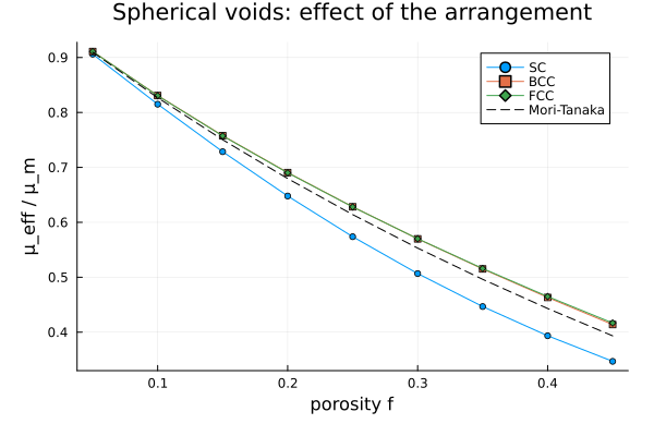
§5 The equivalent inclusion method gives the same answer
On a periodic assembly the two N-body schemes of the package are the same linear system — the identity Brisard et al. (2014) state in their §3.1, their order-zero influence pseudotensors being the interaction tensors of El Mouden. They agree to machine precision, which is the acceptance gate of both implementations.
println("\n  cutoff    cluster        EIM            max|difference|")
for c in (0.0, 1.5, 3.0)
    asm = cubic_lattice(:sc, Dict(:C => C_m), Dict(:C => C_rigid); fraction = 0.3, cutoff = c)
    A = get_array(homogenize(asm, ClusterModel(), :C))
    B = get_array(homogenize(asm, EquivalentInclusion(), :C))
    @printf "   %.1f     %.10f   %.10f   %.2e\n" c A[1, 2, 1, 2] B[1, 2, 1, 2] maximum(abs.(A .- B))
end

p_full = plot(p1, p2, p3; layout = (1, 3), left_margin = 8Plots.mm, bottom_margin = 8Plots.mm,
    size = (1500, 520), titlefontsize = 9)
p_full
This page was generated using Literate.jl.