The Laplace-Carson route

Linear viscoelasticity comes in two flavors, and MeanFieldHomogenization implements both by entirely separate means.

When the material's properties do not depend on the age of the specimen — only on the elapsed time since loading — the constitutive law is a convolution, and a transform turns it into a product. That is the Laplace-Carson route of this page: the correspondence principle reduces the whole viscoelastic homogenization problem to an elastic one at each value of a transform variable, solved by the ordinary homogenize machinery, with a numerical inversion to come back to the time domain.

When the properties do depend on age — concrete that is still hydrating, a gel whose volume fraction grows — no transform helps, and the Volterra operators have to be discretized directly. That is the ageing route, which is strictly more general and correspondingly more expensive.

The two are related the way a Fourier method is related to a time-stepping scheme: the transform route is cheaper and more accurate where it applies, the direct route applies always. For a non-ageing material they must agree, and the three-route comparison checks that they do.

The transform, and why Carson rather than Laplace

The Laplace-Carson transform of a function of time is its Laplace transform multiplied by the transform variable:

The extra factor p is what makes the convention worth having: it maps a constant to itself,

so an elastic modulus is its own transform. Everything written for elasticity carries over to the transform domain with no bookkeeping factor: a stiffness stays a stiffness, a Hill tensor stays a Hill tensor, a volume fraction stays a volume fraction.

Two elementary pairs generate most of what the model catalog needs:

		appears in
		every elastic channel
		a Maxwell branch
		a Kelvin branch
		a series dashpot
		a parabolic (springpot) element
		the fractional Zener and Rabotnov kernels
		logarithmic creep

The fifth line is the one that does the most work: it is why ScottBlair, HuetSayegh and Model2S2P1D are elementary in both domains, and hence why 2S2P1D can drive the Volterra route and the transform route with no approximation on either side.

The correspondence principle

The non-ageing constitutive law is the Stieltjes convolution

whose Laplace-Carson transform is a plain product,

Transformed, the field equations of the localization problem — equilibrium, compatibility, the interface conditions — are identical to those of an elastic problem whose stiffness is , with p a parameter. Therefore

every homogenization scheme, applied at fixed p to the transformed moduli, yields the transform of the effective relaxation tensor.

In practice this means the viscoelastic problem is solved by code that knows nothing about viscoelasticity. MeanFieldHomogenization needs no separate scheme implementations for the Laplace-Carson route: the elastic ones are used unchanged, and the only requirement is that they be generic in the scalar type — which they are, and which test/Schemes/test_complex_moduli.jl pins down.

homogenize_lc is the thin driver around that observation.

It is the non-ageing case only

The step from convolution to product needs the kernel to depend on t - s alone. A kernel R(t, t') with genuine age dependence has no such factorization, and no amount of care with the transform recovers it. For those materials, homogenize_alv is the answer, not this page.

Creep and relaxation: a product here, a convolution there

The single most useful consequence of the transform is that creep and relaxation, which are related by a convolution in time,

become exact reciprocals in the transform domain:

That identity is what carson_creep exploits as its default implementation, and it is what makes the Kelvin ⇄ Maxwell conversion of the next section possible at all.

The same asymmetry explains why a viscoelastic Poisson ratio is a Laplace-Carson object: 3k* = E*/(1-2ν*) is a pointwise identity in p, but in the time domain the corresponding relation is a Volterra quotient — ν(t) does not divide, it deconvolves. YoungPoisson carries that caveat.

Interlacing: why Kelvin ⇄ Maxwell is exact

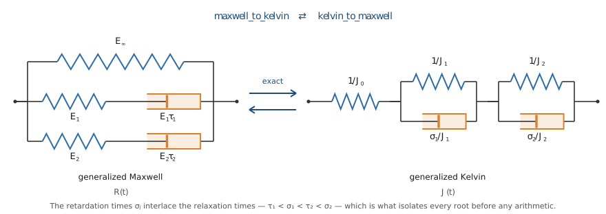
A generalized Maxwell chain and a generalized Kelvin chain describe the same material. Since

is a rational function of p, and J* = 1/R*, converting between the two representations is a partial-fraction decomposition. The reference implementation in ECHOES does exactly that symbolically: expand   into a polynomial and root-find. That is correct and it is badly conditioned — real relaxation spectra carry dozens of branches over six to ten decades, and such a polynomial cannot be formed in floating point without losing its roots.

There is far more structure available than "the roots of a polynomial". Write   . Then

for a positive spectrum. Φ is a Stieltjes function: strictly increasing between consecutive poles, running from -∞ to +∞ across every gap. Counting sign changes gives the zeros exactly, and they interlace the poles:

     0  <  τ₁  <  σ₁  <  τ₂  <  σ₂  <  …  <  τ_m  <  [σ_m]

with the last zero present iff  . There is deliberately no zero in : Φ(0⁺) is the glassy modulus, which is positive, and Φ only increases from there.

The dual direction is not symmetric, and this is the one place an implementation must not assume it is. With

Ψ(0⁺) = J_0 > 0 while Ψ(τ₁⁻) = -∞, so there is a zero below the first pole:

     0  <  σ₁  <  τ₁  <  σ₂  <  τ₂  <  …  <  τ_n  <  [σ_{n+1}]

the last one existing iff the fluidity  . Hence a solid Kelvin chain with n branches converts to n Maxwell branches with  , while a fluid one converts to n+1 branches with   — which is the degree count of the rational transform, as it must be.

Each unknown is thus isolated before any arithmetic happens. Bisection in log σ then cannot fail, whatever the number of branches or their spread, and the residues

are positive by construction rather than by luck, because Φ' > 0 and Ψ' < 0. maxwell_to_kelvin and kelvin_to_maxwell implement this; the tutorial draws the interlacing and shows the round trip staying at 1e-15 out to twenty branches.

The degenerate branches

A material with no equilibrium spring — a fluid — has its outermost zero at infinity. That is not a failure mode to guard against; it is the series dashpot of the Kelvin form, and it is recovered exactly as

Because of this, PronyCreep stores a fluidity   rather than a viscosity, and both Prony types keep their degenerate branches in named scalar fields rather than inside the τ vector. The reason is not aesthetic: Inf inside a vector that is then sorted, exponentiated and differentiated produces NaN partials under ForwardDiff, whereas 0 behaves like any other number.

Inversion: the hard direction

Going to the transform domain is a quadrature. Coming back is not: the transform smooths, so inverting it amplifies whatever is left of the arithmetic. There is no way around this, only algorithms with different trade-offs, and MeanFieldHomogenization ships four of them — see the manual page for how to choose and the tutorial for the measurements.

Three properties are worth knowing before reading any of them.

Accuracy is absolute, not relative. Every method controls its error against the scale of f, not against f(t) at the point asked for. Once a relaxation function has decayed many orders of magnitude below its initial value, the relative error is unbounded while the absolute one still meets the method's promise. This is intrinsic, and it is why a viscoelastic solid — whose relaxation function settles on a plateau   — is the comfortable case, and a fluid's tail must be read as an absolute quantity.

The choice of nodes decides what the transform must support. Three of the four algorithms place their nodes off the real axis, so the transform must accept complex arguments. GaverStehfest does not: its nodes are real and positive. That is a genuine architectural property rather than a detail — it means a whole homogenize_lc sweep runs in real arithmetic, which halves the cost of each scheme evaluation and is the only way to use SelfConsistent(algorithm = NewtonDefault()) on this route, since its ForwardDiff Jacobian cannot carry a Dual over a complex scalar.

Branch cuts are not the obstacle one expects. The Talbot contours are Hankel-shaped: they wrap around the negative real axis rather than crossing it, which is precisely how they were designed to handle singularities there. Every fractional model in the catalog inverts at full accuracy under them. What actually separates the algorithms is oscillation — a rotating phase is invisible to a method whose nodes are all real.

Collocation: inversion by fitting

There is a fifth route that is not a quadrature at all. Given any transform, prony_fit_relaxation fits a Prony series to it by least squares on a set of collocation points — the Schapery method. The result is not an approximation of f(t) at one point but a model: it has a closed-form time function, an exact dual chain through the conversion above, a ViscoLaw for the ageing pipeline, and derivatives.

Fitting with a non-negativity constraint on the spectrum is what keeps the result completely monotone, hence passive. It is also, empirically, the better fit: on a fractional Zener model the constrained fit is three times more accurate on the master curve than the unconstrained one, which puts half its moduli below zero.

Where each piece lives

the transform of a model	carson_relaxation, carson_creep — catalog
back to the time domain	inverse_carson — manual
the exact chain conversion	maxwell_to_kelvin, kelvin_to_maxwell
fitting a chain to a transform	prony_fit_relaxation, prony_fit_creep
homogenizing on this route	homogenize_lc
the ageing alternative	homogenize_alv — theory