The differential scheme

The differential (or incremental) scheme builds the composite by repeated dilute incorporation: an infinitesimal amount of each inclusion phase is added to the current effective medium, which is re-homogenized before the next increment. This page derives the resulting ODE for an arbitrary number of phases and an arbitrary incorporation trajectory ([31]).

Incorporation process

The construction is a loop, and the loop is the scheme: what distinguishes it from Mori–Tanaka is not the dilute step — that step is the same — but the fact that the reference medium is updated after each one.

Two things in that loop are worth naming before the algebra: the increments are taken out of the current medium, not out of the original matrix, and the order in which the phases are grown is a free choice — the trajectory. Both are what makes the scheme path-dependent.

The RVE holds a matrix (index 0) and N inclusion phases, of final volume fractions . Each phase is grown along a fictitious incorporation time,

non-decreasing, the matrix taking up the rest,

Between and  , a volume fraction of the current medium is replaced by phase i. The are the increments the scheme actually applies; the are what the user prescribes. They differ, because removing of the current medium also removes the phase i already present in it:

In matrix form, with  ,

The matrix to invert is a rank-one update of the identity, so the Sherman-Morrison formula gives the inverse in closed form:

that is, component-wise,

This is exactly what the RHS of the scheme evaluates at every step (_diff_ode_rhs! in src/Schemes/differential.jl); nothing else about the trajectory enters the volume balance.

The derivation above assumes every phase occupies a finite volume. Crack families do not, and the balance has to be extended — see the section on cracks below.

The ODE

The incremental step replaces of the current medium by phase i, each increment being a dilute problem posed in that medium:

where is the size-independent stiffness contribution of phase i in the current medium,

Written this way, needs only the phase's concentration tensors — not a Hill tensor, and not even a uniform phase property. It is therefore available for every inclusion family the package supports (ellipsoids, cylinders, flat cracks, multi-layer spheres and spheroids), which is why the differential scheme accepts all of them without special-casing. See Localization.

Hence the ODE integrated by DifferentialScheme:

started from  . The package parametrizes the incorporation time as   .

Compliance form

The same process written on the compliance uses the compliance contribution of each phase:

The two forms are exactly equivalent: the second is the image of the first under  , term by term. They are not numerically identical, though — the solver controls its error on whichever variable is integrated. The compliance form is better conditioned for a medium that softens towards percolation (porous or cracked), the stiffness form for one that stiffens. Both are available through the formulation keyword and can be compared on the same RVE:

homogenize(rve, DifferentialScheme(), :C)                             # stiffness
homogenize(rve, DifferentialScheme(; formulation = :compliance), :C)  # compliance

Cracks: a departure from the volume-replacement picture

Flat cracks do not fit the derivation above, and the difference is physical rather than technical. A penny-shaped crack of radius a and aperture c has, for an aspect ratio   ,

( cracks of that family in the volume )

so its volume fraction vanishes asymptotically while its density stays finite — and it is the density, not the fraction, that measures the mechanical effect. Three consequences for the scheme:

1. The volume balance must be rewritten. Opening a crack removes no current medium, so cracks do not appear in the sum and

   whatever the crack densities ( = solid phases). They are nevertheless diluted by it: the piece of current medium that gets replaced by solid material takes the cracks it contained with it, and the incoming material has none. Writing for the density of cracks actually created in the current medium,

   Both lines are the single rank-one relation     on the stacked amounts  , where carries a 1 on solid entries and a 0 on crack entries — the only change to the manuscript's derivation. The same Sherman-Morrison inverse follows, with the density playing the role of the fraction:

   and the crack term of the ODE is

   The crack correction vanishes whenever no solid phase grows at the same τ — a crack-only RVE, or a Sequential trajectory in which the cracks come after the solids — and is what makes mean the density actually reached at τ, consistently with for solids.

2. There is no saturation from the volume side. A solid phase is bounded by  ; a crack density is not, so nothing geometric stops the integration — f₀ is still 1 at any density. The effective stiffness decays towards zero asymptotically in without a finite threshold, unlike the self-consistent scheme, because each infinitesimal crack increment is introduced into an already-degraded medium.

3. The compliance form is the natural one. As   the crack's strain concentration tensor diverges, so the stiffness contribution is a limit of a divergent quantity, while the compliance contribution — built from the crack-opening-displacement tensor, see COD tensors — stays finite and is what the package actually computes:

   with the Budiansky-O'Connell prefactor (4π/3 for 3D penny and elliptic cracks, π for 2D ribbons). The stiffness form of the ODE therefore evaluates the crack term by passing through anyway; formulation = :compliance merely stops undoing that conversion, which is why it behaves better on heavily cracked media.

Apart from that, cracks follow the chosen trajectory exactly like solid phases, through : Proportional, Sequential and the explicit paths all apply to a CrackDensity amount, the target being the final density instead of the final volume fraction.

Trajectories

With a single inclusion phase the trajectory is immaterial: any monotone traverses the same states, and only the final fraction matters. With two or more phases, the order of incorporation is a modeling choice — the effective property at τ = 1 depends on it. Three cases, following the same order as the derivation above.

1. Homothetic growth

All phases grow proportionally,    with  ,   (the default Proportional, where  ). Then     and

This closed form is a useful check on the volume balance alone, independently of any tensor algebra; the single-phase case reduces to the classical    .

2. Successive phases

Each phase is grown to completion before the next one starts — Sequential, given the incorporation order. Phase i owns a contiguous slice of τ and is frozen outside it.

3. Arbitrary trajectory

The user prescribes for every inclusion phase and    follows — Path for callables (differentiated by ForwardDiff) or CustomPath for tabulated values (piecewise-linear):

DifferentialScheme(; trajectory = Path(:I1 => τ -> τ^2, :I2 => τ -> 2τ - τ^2))

The three, side by side

For two phases the trajectory is a curve in the 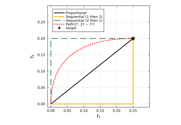plane. All four curves below start at the origin and end at the same target   — so they describe the same material, and they will not give the same effective stiffness:

They all agree in the dilute limit — near the origin every curve is tangent to its own straight line and the first-order term is the same — and they separate like at finite fractions. The spread is a feature of the scheme, not a numerical artifact: it is what makes the differential scheme able to represent a processing history, and it is measured in Comparing loading-path trajectories.

Conduction and viscoelasticity

The derivation never used the tensor order: replacing by gives the conduction / diffusion scheme, and the compliance form becomes the resistivity form. Both orders are implemented.

In ageing linear viscoelasticity the same ODE holds on the discrete Volterra block matrices, the products being Volterra products (differential_alv for the relaxation tensor, differential_alv_order2 for conduction) — see Viscoelasticity. One restriction is specific to ALV: the ALV Hill kernel is built for an isotropic reference, and the reference of the differential scheme is its running medium, so every phase must keep that medium isotropic (spherical inclusions, multi-layer spheres, or any shape with symmetrize = :iso). The ODE raises an explicit error otherwise.

Numerical resolution

The ODE is integrated by OrdinaryDiffEq.solve, adaptive Tsit5 by default; the algorithm and its tolerances are user-facing — see Homogenization schemes for the keywords.

Two things about it are theory rather than plumbing.

The state is sized by the running estimate, not by the matrix. It carries the canonical components in the smallest symmetry class that estimate can stay in — two numbers for an isotropic medium, five to eight for a transversely isotropic one, the full Mandel matrix otherwise. A phase whose contribution is less symmetric drags the estimate out of the matrix's class at the first step (a crack, or simply an aligned spheroid, whose is transversely isotropic even between two isotropic materials), so the scheme probes each contribution once before integrating.

The residue algorithm cannot be used here. When the running estimate is anisotropic from the first step, the Hill tensors are evaluated by cubature: the acoustic polynomial of the residue method degenerates precisely at the isotropic starting point of the integration. That is what method = :auto selects, and an explicit method = :residues on such an RVE raises an error saying so.