
A layered spheroid, meshed
N nested coaxial spheroids in an isotropic matrix, solved by Fourier axisymmetric finite elements — and checked against the two closed forms this package already carries. The method is the finite Eshelby cell; how to call it is Finite-element inclusions.
This page is static
The figures and the numbers are produced once by scripts/fe/make_layered_spheroid_figures.jl and committed. No finite element runs at documentation-build time: the documentation environment carries neither Ferrite nor gmsh, on purpose.
Why mesh a body that has a closed form
Because most of them do not. The confocal multilayer spheroid has an analytic solution — LayeredSpheroid, in both physics — and a nest of spheroids with freely chosen semi-axes has none. The finite-element cell covers both, which means the case with a closed form is not a demonstration but a calibration: it is where the solver can be told it is right, on a body whose answer is known.
So this page does the two in order. First the slices with an exact answer, to fix how much to trust the cell. Then the geometry no closed form reaches.
The geometry is the analytic type's, not a transcription of it
Layers are given by their semi-axes, per layer, ascending: the same (axis_radii, disk_radii) pair LayeredSpheroid takes, in the same order. One call produces them and both inclusions consume them:
using MeanFieldHomogenization, TensND
import Ferrite, FerriteGmsh, Gmsh                    # the backend

ar, dr = confocal_layer_radii(2.0, 1.0, (0.3, 0.7))  # ω = 2, core 30 % of the volume
K = (TensISO{3}(5.0), TensISO{3}(2.0))               # core, then shell

fe  = FEAxiLayeredSpheroid(ar, dr, K)
ana = LayeredSpheroid(ar, dr, K)                     # the same body, in closed form
That matters more than it looks. A cross-check is only worth something if the two solvers are handed the same body; describing the geometry twice — once as (focal, q) and once as semi-axes — is how a comparison ends up measuring a transcription error and calling it a discretization error.
The mesh
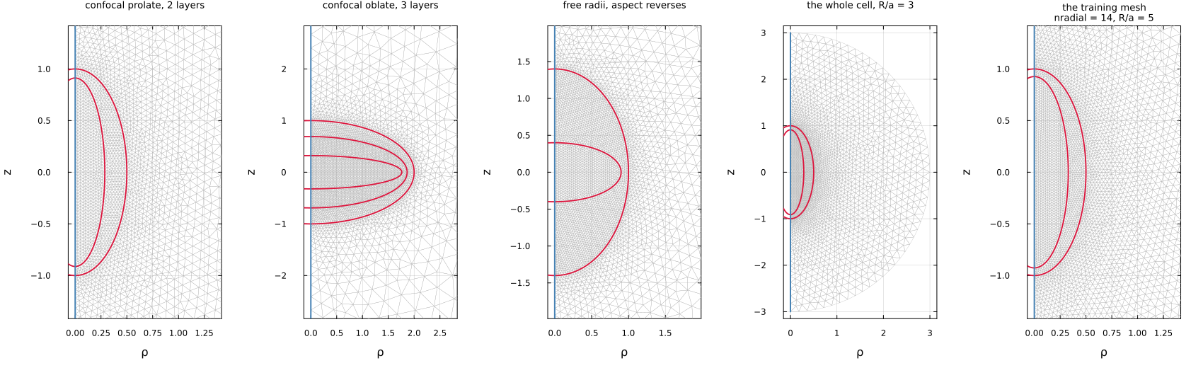
Being two-dimensional, this is the whole computational domain and not a slice of one. Each layer boundary is drawn in crimson from its own closed form rather than from the mesh, and the revolution axis in blue. The first three panels are zoomed on the inclusion; the fourth is the same first case at full extent, showing where the matrix ends and the corrected boundary condition acts.
The third panel is the one to look at: an oblate core inside a prolate shell. It is nested, it is axisymmetric, and no confocal family contains it — confocal spheroids share their foci, so the outer layer is always rounder than the core. That panel is what the finite elements are for.
| geometry | layers | cells | worst layer volume error |
|---|---|---|---|
| confocal prolate, 2 layers | 2 | 5985 | 4.8e-04 |
| confocal oblate, 3 layers | 3 | 7947 | 7.2e-04 |
| free radii, aspect reverses | 2 | 7550 | 9.4e-04 |
The volume column is the check that is available on any geometry, confocal or not: each layer's meshed volume of revolution against the closed form
The fifth panel is not an illustration: it is the discretization every training label was computed on — nradial = 14, R/a = 5, 11 030 cells at the middle of the sampling box. The four to its left use nradial = 16 and R/a = 3 because that reads better on a page, so without the fifth one the mesh the shipped surrogates actually learned from would appear nowhere.
Against the two closed forms
The space of nested spheroids is a two-parameter family per layer, and it is crossed by two independent exact slices which meet only at the equal-radii sphere:
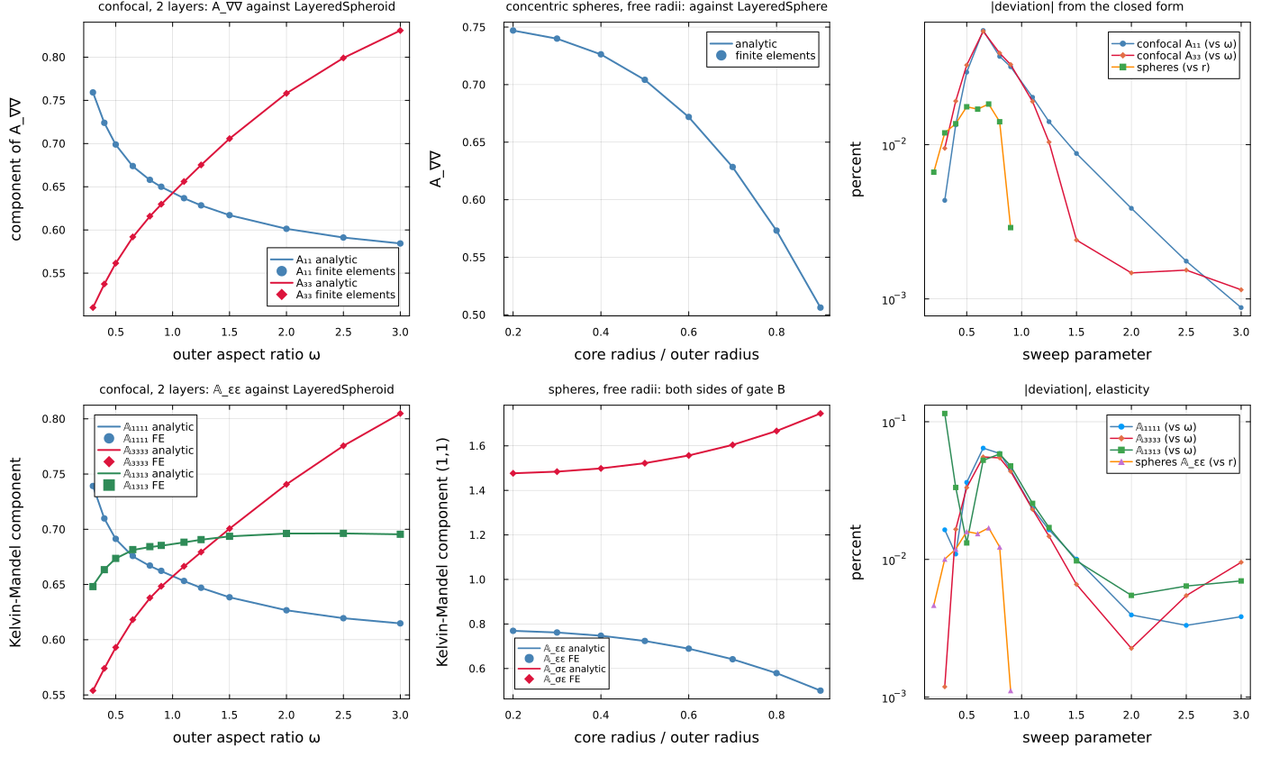
The left panel sweeps the outer aspect ratio from LayeredSpheroid. Both branches of that solution are exercised on one curve, and deliberately: the oblate branch runs the whole computation in complex arithmetic — the substitution
The middle panel is concentric spheres of arbitrary radii, against LayeredSphere. This slice is not confocal at all, which is what makes it valuable: it covers an arbitrary layer count and freely chosen radii without assuming the confocal relation anywhere.
The top row is conduction and the bottom row elasticity; the right-hand panels collect the deviations. Everything is below
Two layers. Conduction: k₁/k₀ = 5, k₂/k₀ = 2. Elasticity: E₁/E₀ = 4, ν₁ = 0.2, E₂/E₀ = 1.5, ν₂ = 0.3, ν₀ = 0.25.
| slice | worst deviation | median deviation |
|---|---|---|
confocal, A₁₁, ω ∈ [0.3, 3] | 5.5e-04 | 1.3e-04 |
confocal, A₃₃, ω ∈ [0.3, 3] | 5.4e-04 | 1.0e-04 |
| spheres, free radii | 1.8e-04 | 1.4e-04 |
confocal, A₁₁₁₁, ω ∈ [0.3, 3] | 6.4e-04 | 1.6e-04 |
confocal, A₃₃₃₃, ω ∈ [0.3, 3] | 5.6e-04 | 1.5e-04 |
confocal, A₁₃₁₃, ω ∈ [0.3, 3] | 1.1e-03 | 1.7e-04 |
confocal, 𝔸_σε — no reference | — | — |
spheres, elasticity, 𝔸_εε | 1.7e-04 | 1.2e-04 |
spheres, elasticity, 𝔸_σε | 9.5e-05 | 7.4e-05 |
Two panels are worth a second look. The conduction components cross at LayeredSphere to
What this comparison found in the analytic solution
The elastic sweep above covers the sphere, and for a while it could not. A one-layer confocal spheroid is a homogeneous spheroid, so the closed-form Eshelby result is its answer and the confocal machinery has to reproduce it at every aspect ratio. It did not: the error went from
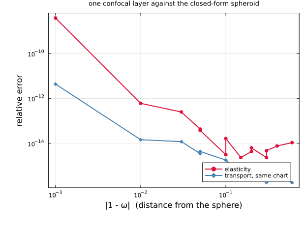
One confocal layer is a homogeneous spheroid, so the closed-form Eshelby result is the reference and the confocal machinery must reproduce it exactly. Transport does, everywhere. Elasticity does not, once the chart degenerates (focal → 0, q → ∞).
ω | elasticity | transport, same chart |
|---|---|---|
| 0.999 | 3.8e-09 | 4.3e-12 |
| 0.990 | 6.0e-13 | 1.4e-14 |
| 0.970 | 2.5e-13 | 1.2e-14 |
| 0.950 | 4.3e-14 | 3.5e-15 |
| 0.900 | 3.1e-15 | 1.8e-15 |
| 0.850 | 2.3e-15 | 4.5e-16 |
| 0.800 | 4.3e-15 | 7.7e-16 |
| 0.700 | 2.3e-15 | 1.8e-16 |
| 0.600 | 7.6e-15 | 3.5e-16 |
| 1.050 | 3.7e-14 | 4.4e-15 |
| 1.100 | 1.6e-14 | 1.8e-15 |
| 1.200 | 6.3e-15 | 9.9e-16 |
| 1.300 | 4.7e-15 | 3.5e-16 |
| 1.600 | 1.1e-14 | 1.8e-16 |
Against the closed forms
Two layers. Conduction: k₁/k₀ = 5, k₂/k₀ = 2. Elasticity: E₁/E₀ = 4, ν₁ = 0.2, E₂/E₀ = 1.5, ν₂ = 0.3, ν₀ = 0.25.
| slice | worst deviation | median deviation |
|---|---|---|
confocal, A₁₁, ω ∈ [0.3, 3] | 5.5e-04 | 1.3e-04 |
confocal, A₃₃, ω ∈ [0.3, 3] | 5.4e-04 | 1.0e-04 |
| spheres, free radii | 1.8e-04 | 1.4e-04 |
confocal, A₁₁₁₁, ω ∈ [0.3, 3] | 6.4e-04 | 1.6e-04 |
confocal, A₃₃₃₃, ω ∈ [0.3, 3] | 5.6e-04 | 1.5e-04 |
confocal, A₁₃₁₃, ω ∈ [0.3, 3] | 1.1e-03 | 1.7e-04 |
confocal, 𝔸_σε — no reference | — | — |
spheres, elasticity, 𝔸_εε | 1.7e-04 | 1.2e-04 |
spheres, elasticity, 𝔸_σε | 9.5e-05 | 7.4e-05 |
The cause was not the geometry and not the layer coupling — one layer already showed it, and both the prolate and the oblate family failed. The columns of the elastic system are amplitudes of Papkovich–Neuber potentials at the interface, so a growing mode of degree
The degeneracy is in the basis's normalization, not in the problem: as
| before | after | |
|---|---|---|
3e-15 | 2e-15 | |
1.6e-3 | 3e-15 | |
5.4e-2 | 4e-14 | |
7.7e-1 | 6e-13 | |
1.0e+0 | 4e-9 |
A residual limit remains at
Nothing caught this before: the failure changes no strain-side result away from the sphere, it is invisible in transport, and no test covered the elastic near-sphere limit. It surfaced because a finite-element cell was asked the same question about the same body — which is the whole reason to have two independent routes, and there is now a regression test on the one-layer oracle at every aspect ratio.
Replaying it with your own radii
This is the part the closed forms do not cover, and the whole reason for the type. Two things to know, and one to be honest about.
The two ways in. confocal_layer_radii for the calibrated slice, and a bare pair of semi-axis tuples for anything else:
# Confocal — the slice with an analytic answer.
ar, dr = confocal_layer_radii(0.5, 1.0, (0.4, 0.6))     # oblate, ω = 0.5
FEAxiLayeredSpheroid(ar, dr, K)

# Free radii — an oblate core in a prolate shell, three layers, whatever you like.
FEAxiLayeredSpheroid((0.4, 1.0, 1.4), (0.9, 0.95, 1.0), (k₁, k₂, k₃))
axis_radii are the semi-axes along the revolution axis and disk_radii those across it, ascending, core first. Get the order wrong and nothing is silently wrong: the nesting check refuses it.
julia> FEAxiLayeredSpheroid((0.5, 1.4), (1.1, 1.0), K)
ERROR: ArgumentError: layers 1 and 2 are not nested: layer 1 is
(disk 1.1, axis 0.5) and layer 2 is (disk 1.0, axis 1.4). Both semi-axes must
grow outwards — a wider core inside a narrower shell is not a nest, whatever
the other semi-axis does.
Two coaxial concentric ellipses are nested if and only if both semi-axes grow outwards, so check_nested_spheroids is two comparisons per layer. It is worth doing rather than trusting: a violation is not a wrong answer but a self-intersecting geometry, which gmsh rejects from deep inside its own pipeline with a message naming neither the layer nor the semi-axis.
The growth has to be strict. Two coinciding boundaries pass every containment argument and carry no volume, but they cannot be meshed: the element size is capped at a fraction of each layer's thickness, so a zero-thickness layer asks for a zero-sized element. A sphere is still a perfectly good layer — that is a == c within one layer, which is unrestricted.
The mesh knobs, in order of importance. radius_ratio before nradial: what remains after the dipole correction is truncation, not discretization.
FEAxiLayeredSpheroid(ar, dr, K; opts = FEAxiMeshOptions(; nradial = 16, radius_ratio = 6.0))nradial sets the element size from the outer transverse semi-axis, and the mesher then caps it per layer against that layer's own thickness — a thin shell is resolved whether you asked for it or not, because an element spanning a whole layer leaves that layer unmeshed while the mesh still looks reasonable. Probe the size before solving on a geometry you have not tried:
r = fe_axi_mesh_report(fe)
r.ncells, r.ncells_by_layer, r.volume_error
volume_error is the largest relative departure of a meshed layer's volume of revolution from its closed form, so it is the one number that catches a layer the mesh failed to resolve — and it is available whether or not the geometry has an analytic solution.
What still validates a case with no analytic counterpart, listed so nobody believes they are without a net:
each layer's meshed volume against
, closed form for any semi-axes — layer_volumesgives the exact side;transverse isotropy about the revolution axis, which holds structurally at any refinement and is therefore free;
the coherence limits: equal moduli across the layers must return the homogeneous spheroid, whose Hill tensor is a closed form, and the package agrees to
mesh convergence, and the
sweep, which is the only test that proves the sign of the dipole correction — a wrong sign leaves exactly twice the truncation bias instead of none, and reads as a mesh that will not converge.
And what is not guaranteed. Off the two exact slices there is no reference, only convergence. In particular a nest whose layers have genuinely different aspect ratios has no closed form in this package and, as far as we know, nowhere else.
It has to arrive in a scheme
Which is the point of all of it. The inclusion is heterogeneous, so it enters through gate B with both localization tensors, and both come out of one solve:
C₀ = iso_stiffness(0.6667, 0.4)                       # E = 1, ν = 0.25
Cs = (iso_stiffness(2.2, 1.67), iso_stiffness(1.1, 0.77))
fe = FEAxiLayeredSpheroid((0.6, 1.0), (0.36, 0.6), Cs)

rve = RVE()
add_phase!(rve, :m, Ellipsoid(1.0), Dict(:C => C₀); fraction = :rest)
add_phase!(rve, :incl, fe, Dict(:C => C₀); fraction = 0.15,
           symmetrize = IsoSymmetrize())
homogenize(rve, MoriTanaka(), :C)
Two things in that snippet are not decoration.
The phase property is a placeholder and is ignored: the constituents live in the geometry object, so pass the matrix's own stiffness and nothing is lost.
IsoSymmetrize() is not optional on the iterative schemes. SelfConsistent, AsymmetricSelfConsistent and DifferentialScheme re-evaluate the inclusion in their own running estimate, which for an oriented spheroid is transversely isotropic — and the dipole boundary condition is the closed-form isotropic field, so the cell refuses an anisotropic reference. The failure is a refusal far from the call site, not a wrong number. One-shot schemes are unaffected.
Voigt and Reuss work without any extra input, because the internal volume fractions are a closed form of the semi-axes; layer_fractions returns them. And the bounds do bracket the estimates, which is checked in the suite rather than assumed.
The surrogate, and the sensitivity it unlocks
Everything above costs a mesh and a factorization per evaluation, and that is what forbids a derivative: the solve runs in Float64 and memoizes on the reference medium alone, so a request for ∂/∂w would come back a silent zero. The type raises instead. A trained network is the way through, and it is trained on the cell, not on a closed form, because half of gate B exists nowhere else — the analytic LayeredSpheroid supplies no stress side at all.
julia --project=scripts/nn scripts/nn/train_layered_spheroid.jl 2800 100Two surrogates come out, layered_spheroid_strain and layered_spheroid_stress, and one solve fills a column of both label matrices. 𝔸_σε is not derivable from 𝔸_εε — the inclusion has more than one constituent — so meshing twice to learn two halves of one solve would have doubled several hours of finite elements for nothing.
Those hours are also why the script checkpoints every label as soon as it exists and recomputes only what is missing on a restart. A Halton point depends on its index alone, never on the sample count, so the index is a stable name for a sample: the set grew 400 → 700 → 1200 → 2000 → 2800 and each step reused everything already paid for, so 2800 samples cost 2800 solves rather than the 7100 the five runs would otherwise have needed. That is also what made it affordable to try a different output specification on the same labels — a re-encoding rather than a re-solve. MFH_NN_MAX_NEW bounds the new solves one process performs per data set, which keeps hours of finite elements a sequence of short runs.
The box, and why every feature is a ratio
| feature | range | what it is |
|---|---|---|
log_aspect | prolate; the oblate family is a second box, trained the same way | |
core_fraction | the core's share of the inclusion's volume, which fixes the confocal radii | |
log_mu_ratio_1 | the core against the matrix | |
log_mu_ratio_2 | the shell against the matrix |
Three decisions rather than defaults.
The features are contrast ratios, never absolute moduli. A heterogeneous morphology carries its constituents inside itself, so its localization depends on the reference medium only through the contrasts — which is why one pair of files serves any ℂ₀ at the trained Poisson ratio, and why a network fed absolute moduli would be spending capacity on a redundancy.
The aspect ratio and the moduli enter in log, the core fraction linearly. A SampleBox is linear, so the feature is the sampling law.
Poisson's ratio is fixed at 0.2 and stated, not swept. The shipped pair is the confocal prolate slice at one Poisson ratio, and guard = :error refuses a query outside the box instead of extrapolating.
Using it
The same three lines as any other inclusion. The morphology parameters go in as shape_params — they are the network's features and the fields the sensitivity API differentiates — and the constituents as properties, which back both the contrast features and the Voigt/Reuss bounds.
strain_s = load_surrogate(model_path("layered_spheroid_strain"))
stress_s = load_surrogate(model_path("layered_spheroid_stress"))

C₁ = iso_stiffness(1.6667, 1.25)             # E₁/E₀ = 3, ν = 0.2
C₂ = iso_stiffness(0.3333, 0.25)             # E₂/E₀ = 0.6

nn = NeuralLocalizationInclusion(
    (1.0, 1.0, 2.0);                         # the aspect ratio, as the semi-axes
    strain = strain_s, stress = stress_s,
    shape_params = (; core_fraction = 0.4),
    fractions = (0.4, 0.6),
    properties = (C₁, C₂),
    guard = :error,
)
Both tensors are supplied, so the inclusion enters gate B on the heterogeneous branch — exactly as the meshed cell does, and the schemes cannot tell them apart.
The semi-axes are not sorted, and that is deliberate
A localization class reads column 3 of the inclusion basis as its symmetry axis, because the morphology it describes may be a sphere whose response is transversely isotropic about a direction the outer shape does not name. NeuralHillInclusion sorts its semi-axes descending, to match the frame its Ellipsoid teacher returns; NeuralLocalizationInclusion must not, or (1, 1, ω) with ω > 1 would sort to (ω, 1, 1), put the revolution axis in column 1, and decode a tensor transversely isotropic about an equatorial direction. That was a real bug, fixed in 0.14.1 and now asserted by a test — it had stayed hidden because every localization surrogate before this one was trained on a sphere, where the sort is the identity.
Three routes, and one of them is exact
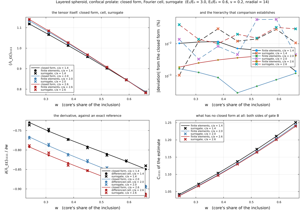
The shipped models cover the confocal slice, and that is worth using rather than hiding: on it 𝔸_εε has a closed form, so the figure judges the cell and the surrogate against an exact answer instead of against each other. Top left, the tensor component by all three routes; top right, the deviation each carries; bottom left, the derivative with respect to the core fraction, again against the exact one; bottom right, the quantity that has no closed form — the effective stiffness, which needs both sides of gate B.
The reference is the closed form differenced at h = 1e-4, and that step is measured rather than assumed: the quotient was checked at 1e-2, 1e-3, 1e-4 and 1e-5 and stops moving at the ninth digit. The surrogate is differentiated by ForwardDiff, so no step size enters on that side; the cell is centrally differenced at h = 2e-2, inside a plateau that was also measured.
Confocal prolate layers, E₁/E₀ = 3.0, E₂/E₀ = 0.6, ν = 0.2, nradial = 14, R/a = 5.0; the core fraction w swept over [0.24, 0.66] at c/a ∈ {1.4, 2, 2.6}, inside the trained box [1.25, 3]. The closed form is the reference where it exists.
| Quantity | vs the closed form, worst over the sweep |
|---|---|
(𝔸_εε)₁₁₁₁, finite elements | 0.01 % |
(𝔸_εε)₁₁₁₁, surrogate | 0.06 % |
∂(𝔸_εε)₁₁₁₁/∂w, differenced cell | 0.087 % |
∂(𝔸_εε)₁₁₁₁/∂w, surrogate | 1.0 % |
At the box boundary c/a = 3.0, the same two quantities: value 0.10 %, derivative 1.2 %.
| Quantity with no closed form | surrogate vs the cell, worst |
|---|---|
C₁₁₁₁ of a Mori-Tanaka estimate, f = 0.30 | 0.02 % |
| Cost of one evaluation | |
|---|---|
| finite elements, cold | 4.717 s |
| surrogate | 4.9 µs |
| speed-up | 968308× |
Why the derivative is the hard part, and what actually moved it
A fit carries a smooth bias of amplitude
What it does respond to is samples, and the amount was measured rather than assumed:
| training solves | value, median / p90 | derivative, median / p90 |
|---|---|---|
| 700 | 1.5e-3 / 1.0e-2 | 2.0e-2 / 2.3e-1 |
| 1200 | 5.0e-4 / 4.2e-3 | 7.5e-3 / 6.1e-2 |
Up to 1200 solves every factor of 1.7 bought close to a factor of three, on the value and on the derivative alike. Beyond that the held-out block error saturates — its exponent falls 2.10 → 0.95 → 0.59 as the bulk of the box reaches the teacher's own floor, the cell being exact only to about 1e-4 itself — while the tail keeps falling for a while longer: from 1200 to 2000 solves the worst derivative over the sweep went 4.4 % to 2.5 %, and at the box face c/a = 3 from 10.9 % to 0.8 %.
From 2000 to 2800 both measures agree that little is left: 2.5 % to 1.0 % on the worst derivative, 0.05 % to 0.06 % on the worst value, 0.8 % to 1.2 % at the box face. Those are maxima over twenty-one points, so a mixture like that is what saturation looks like. Past roughly 2000 solves, more samples stop paying.
The split is still worth carrying away, because between 1200 and 2000 reading either number alone gave the wrong answer: added samples land where a Halton set is sparsest — the faces of the box, not the bulk the held-out set measures.
That last normalization is a decision, not a convenience. Of the 175 grid points, 70 have layers of equal modulus — the inclusion is then homogeneous, 𝔸_εε does not depend on w at all, and the exact derivative is identically zero. A ratio to it is meaningless, the same trap validate_surrogate guards against for sign-crossing components, so the scale is the rms of the exact derivative over the grid, 0.68.
Read it as a heavy tail rather than as one figure: a couple of percent typically, and much worse near the faces of the box and at the strongest contrast pairs. That is enough to drive a gradient-based search, and it is not a substitute for the closed form where one exists.
Two things that would not have helped, both checked
More capacity. The fit's residual was swept on a fine grid of 25 values of w and is smooth and monotone, with no ripple: the network was never over-fitting, so a wider one would have changed nothing. Samples were the lever, three times over.
An anchored baseline. AnchoredHill learns a correction to a closed form instead of the whole tensor, and a layered spheroid has a close one — the homogeneous spheroid at the layers' mean modulus, exact on the whole face r₁ = r₂. It was implemented, trained on the very same labels, and it does not pay: marginally better at the median, 3.5× worse at p90, and worse on the derivative at every quantile. Near the exact face the target is 𝕄 ≈ 𝕀, whose off-diagonal Walpole components are zero, so the anchor manufactures zeros exactly where it is perfect and the tail pays. The baseline ships, tested, so the measurement is reproducible; the shipped models stay DimensionlessHill.
Blaming the reference. The mesher caps element size at a fraction of each layer's thickness, and that thickness moves with w, so a staircase in the cell's response was a real possibility: a differenced cell would then have been measuring its own remeshing. Checked on those same 25 values — the cell count grows smoothly from 10 066 to 12 336, the response has no steps, and the differenced cell agrees with the exact derivative to 1e-4. The cell is an excellent derivative; it is simply an expensive one.
So what is the surrogate for
Not for replacing the closed form where one exists. For the two things that have none, both in the figure's bottom-right panel:
the stress side
𝔸_σε, which the analyticLayeredSpheroiddoes not supply — half of gate B exists only through the cell, and therefore only through something trained on it;the nests the confocal family does not contain, where there is no reference to differentiate at all.
And for cost, and for the sensitivity itself: microseconds against seconds, and a derivative where the cell refuses to give one rather than return the silent zero its memoized Float64 solve would produce.
The whole computation end to end is scripts/94_fe_neural_layered_spheroid.jl; the figure and the table above come from scripts/nn/make_layered_spheroid_figures.jl, both run by hand so that no documentation build meshes or trains anything.
What is not implemented
Imperfect interfaces. The axisymmetric formulation has no displacement- or temperature-jump term at all — the only jump in the package is the three-dimensional crack's — so a spring, membrane, Kapitza or surface-conductive layer is refused by name at construction rather than accepted and ignored:
julia> FEAxiLayeredSpheroid(ar, dr, K; interfaces = (KapitzaInterface(0.1), PerfectInterface{Float64}()))
ERROR: ArgumentError: layer 1 carries a KapitzaInterface, and the axisymmetric
finite-element cell implements `PerfectInterface` only. …
That is the next piece of work, and it is a whole one: a new backend generic, node duplication on the interface trace, and the local normal/tangent frame along a curved meridian. Note that the analytic side is not complete either — LayeredSpheroid supports Kapitza and surface-conductive interfaces in conduction, but PerfectInterface only in elasticity — so an imperfect interface on a spheroid in elasticity is a case with no reference at all, which is exactly where the finite elements would stop calibrating and start providing.
And an equivalent thin layer is not an ellipse
The tempting shortcut is to replace the interface by a thin coating that the mesher can already handle. It does not work as stated, and the reason is geometric rather than numerical: an imperfect interface carries a uniform resistance per unit area, so its equivalent layer must have constant thickness — and the inner boundary of a constant-thickness coating on an ellipse is the offset curve, which is neither confocal, nor similar, nor an ellipse at all. See [36], whose subject is precisely the notion of an equivalent particle.
Shrinking both semi-axes by the same amount does give an ellipse, but its normal distance to the original varies along the meridian, so the equivalent resistance is not uniform and the comparison measures nothing. Doing it properly needs the mesher to accept an arbitrary profile per layer, and a validity limit: an inward offset of distance t self-intersects once t exceeds the smallest radius of curvature,
Sensitivities, from the cell itself. The solve runs in Float64 and memoizes on the reference medium, so a derivative with respect to a layer radius or a core fraction would come back a silent zero; the type raises instead. That is what the surrogate above is for, and the same route serves the concave pores.
See also
The finite Eshelby cell — the correction, and why the solid declination uses both outputs of its fixed point.
Finite-element inclusions — the shared syntax.
The confocal layered spheroid — the closed form this page is calibrated against.
Concave pores — the axisymmetric cavity, and the same cell with one region instead of
N.