The rheological model catalog

A linear viscoelastic material can be described by any one of four functions — the relaxation modulus R(t), the creep compliance J(t), and their Laplace-Carson transforms R*(p) and J*(p) — and the four are equivalent. Which one is elementary, though, depends entirely on the model: a Prony series is a sum of exponentials in time and a sum of simple fractions in p, whereas 2S2P1D is a two-line formula in p and has no closed form in time at all.

The catalog is built around that asymmetry. A model states its carson_relaxation — the one method it must provide — plus whichever of the other three it happens to know, and the rest are supplied by exact algebra (J* = 1/R*) or by numerical inversion. Every model therefore answers all five generics whatever it declared, so downstream code never has to ask which.

This page walks the catalog and then shows the two things it is for: lifting a pair of scalar models to an isotropic tensor, and driving both homogenization routes from one object.

using MeanFieldHomogenization
using TensND
using Printf
using Plots
gr()  # headless backend; GKSwstype is set to "100" before Literate runs

Plots.GRBackend()

§1 The classical chains

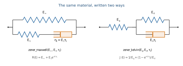
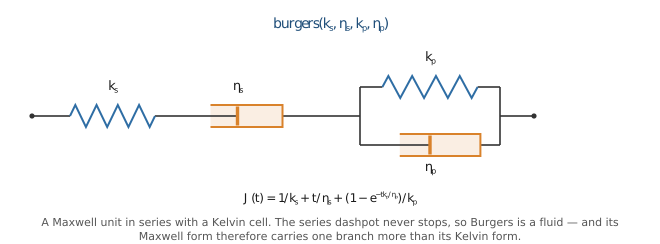
zener_maxwell and zener_kelvin are the standard linear solid written the two ways round; burgers adds a series dashpot and turns it into a fluid; PronyRelaxation generalizes to any number of branches. All four are exact in all four functions, because maxwell_to_kelvin supplies whichever chain the model was not given in.

ts = exp10.(range(-2, 3; length = 300))

classical = [
    ("Zener (standard solid)", zener_maxwell(2.0, 5.0, 1.0), :crimson),
    ("Burgers (fluid)", burgers(1.0, 3.0, 2.0, 6.0), :darkorange),
    ("Prony, 4 branches", PronyRelaxation(1.0, [2.0, 1.5, 1.0, 0.8], [0.05, 0.5, 5.0, 50.0]), :seagreen),
]

p_classical_R = plot(
    xscale = :log10, xlabel = "t", ylabel = "R(t)", legend = :bottomleft,
    title = "relaxation modulus"
)
p_classical_J = plot(
    xscale = :log10, yscale = :log10, xlabel = "t", ylabel = "J(t)",
    legend = :topleft, title = "creep compliance"
)
for (name, m, col) in classical
    plot!(p_classical_R, ts, [relaxation(m, t) for t in ts]; lw = 2.5, color = col, label = name)
    plot!(p_classical_J, ts, [creep(m, t) for t in ts]; lw = 2.5, color = col, label = name)
end

The Burgers curve is the one that goes to zero on the left panel and grows without bound on the right: that is what is_fluid reports, and it is the same fact seen twice.

for (name, m, _) in classical
    @printf "%-24s fluid: %-5s  E_glassy = %8.4f  E_∞ = %8.4f\n" name is_fluid(m) glassy_modulus(m) equilibrium_modulus(m)
end

Zener (standard solid)   fluid: false  E_glassy =   7.0000  E_∞ =   2.0000
Burgers (fluid)          fluid: true   E_glassy =   1.0000  E_∞ =   0.0000
Prony, 4 branches        fluid: false  E_glassy =   6.3000  E_∞ =   1.0000

§2 The fractional family

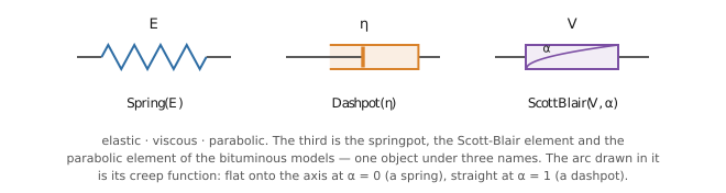
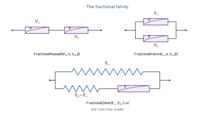
A single exponential gives a relaxation spectrum one decade wide. Real polymers and bitumen relax over six or more, which is what the fractional elements are for: ScottBlair interpolates continuously between a spring (α = 0) and a dashpot (α = 1), and FractionalZener — the Cole-Cole model — replaces the single exponential of a Zener element by a Mittag-Leffler function, broadening the transition without adding branches.

p_fractional = plot(
    xscale = :log10, yscale = :log10, xlabel = "t", ylabel = "R(t)",
    legend = :bottomleft, title = "broadening a Zener transition"
)
plot!(p_fractional, ts, [relaxation(zener_maxwell(2.0, 8.0, 1.0), t) for t in ts]; lw = 3, color = :black, label = "Zener (α = 1)")
for (α, col) in ((0.8, :royalblue), (0.6, :purple), (0.4, :magenta))
    fz = FractionalZener(2.0, 10.0, 1.0, α)
    plot!(p_fractional, ts, [relaxation(fz, t) for t in ts]; lw = 2, color = col, label = "FractionalZener, α = $α")
end

ScottBlair is the one model whose four functions are all closed form and none of them bounded — the exact pair     is what makes the power-law terms of the bituminous models analytic in both domains.

sb = ScottBlair(1.7, 0.4)
for t in (0.01, 1.0, 100.0)
    @printf "ScottBlair  t=%7.2f   J(t) closed form %.10f   by inversion %.10f\n" t creep(sb, t) inverse_carson(p -> carson_creep(sb, p), t)
end

ScottBlair  t=   0.01   J(t) closed form 0.1050747359   by inversion 0.1050747359
ScottBlair  t=   1.00   J(t) closed form 0.6629767635   by inversion 0.6629767635
ScottBlair  t= 100.00   J(t) closed form 4.1831005816   by inversion 4.1831005816

§3 Bituminous binders: Huet-Sayegh and 2S2P1D

Model2S2P1D — 2 Springs, 2 Parabolic elements, 1 Dashpot — is the reference model for bituminous binders and mixtures. HuetSayegh is the same object without the series dashpot, hence a solid rather than a fluid.

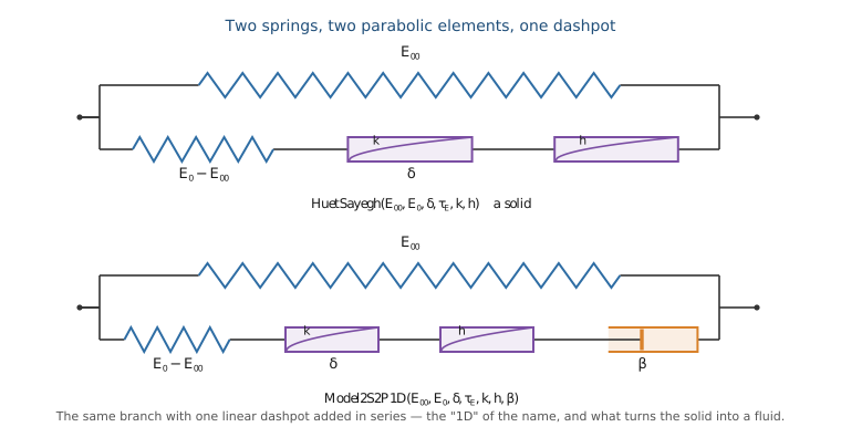
The natural way to look at either is not R(t) but the complex modulus E*(ω), which is what a dynamic test measures. Two conventional plots: the Cole-Cole diagram, plotting the loss modulus against the storage modulus, and the Black diagram, plotting the norm of E* against its phase angle. Both collapse the frequency axis, which is why they are used to check a fit.

binder = Model2S2P1D(1.0e-7, 1000.0, 2.2, 1.94507827e-3, 0.22, 0.63, 50.0)
mix = Model2S2P1D(86.3470095, 26000.0, 2.52254414, 0.834764484, 0.22, 0.65, 43.3031679)
hs = HuetSayegh(20.0, 25000.0, 2.5, 0.8, 0.22, 0.65)

ωs = exp10.(range(-6, 8; length = 400))

p_master = plot(
    xscale = :log10, yscale = :log10, xlabel = "ω  (rad/s)", ylabel = "|E*(ω)|",
    legend = :bottomright, title = "master curves"
)
for (name, m, col) in (("binder (2S2P1D)", binder, :darkorange), ("mix (2S2P1D)", mix, :navy), ("Huet-Sayegh", hs, :seagreen))
    plot!(p_master, ωs, [abs(complex_modulus(m, w)) for w in ωs]; lw = 2.5, color = col, label = name)
end

p_colecole = plot(
    xlabel = "E′(ω)  — storage", ylabel = "E″(ω)  — loss",
    legend = :topleft, title = "Cole-Cole"
)
for (name, m, col) in (("mix (2S2P1D)", mix, :navy), ("Huet-Sayegh", hs, :seagreen))
    plot!(
        p_colecole,
        [storage_modulus(m, w) for w in ωs], [loss_modulus(m, w) for w in ωs];
        lw = 2.5, color = col, label = name
    )
end

p_black = plot(
    xlabel = "phase angle  (degrees)", ylabel = "|E*(ω)|", yscale = :log10,
    legend = :topright, title = "Black diagram"
)
for (name, m, col) in (("mix (2S2P1D)", mix, :navy), ("Huet-Sayegh", hs, :seagreen))
    plot!(
        p_black,
        [rad2deg(angle(complex_modulus(m, w))) for w in ωs],
        [abs(complex_modulus(m, w)) for w in ωs];
        lw = 2.5, color = col, label = name
    )
end

2S2P1D is exact in both domains

The 2S2P1D transform is E00 + (E0 - E00)/φ*(p), and its denominator is the Laplace-Carson transform of an ordinary function of time, term by term:

So the same model is an exact Laplace-Carson object and an exact Volterra object: creep_kernel gives , carson_creep_kernel gives , and creep_kernel_law packages the former as a ViscoLaw for the ageing pipeline. Inverting one must reproduce the other:

for t in (1.0e-5, 1.0e-3, 1.0e-1, 10.0)
    exact = creep_kernel(binder, t)
    inverted = inverse_carson(p -> carson_creep_kernel(binder, p), t)
    @printf "φ(%8.1e) : closed form %.10f   by inversion %.10f   (rel %.1e)\n" t exact inverted (abs(inverted - exact) / exact)
end

φ( 1.0e-05) : closed form 1.7960555110   by inversion 1.7960555110   (rel 9.5e-13)
φ( 1.0e-03) : closed form 3.8245095924   by inversion 3.8245095924   (rel 3.5e-13)
φ( 1.0e-01) : closed form 21.0976461894   by inversion 21.0976461894   (rel 2.3e-13)
φ( 1.0e+01) : closed form 362.3058821548   by inversion 362.3058821549   (rel 1.4e-13)

§4 One object, two routes

iso_rheology pairs two scalar models into an isotropic fourth-order model — here an elastic bulk modulus and a 2S2P1D shear channel. The single object then yields

• p -> carson_relaxation(m, p), which any scheme homogenizes through homogenize_lc;

• ViscoLaw(m), which homogenize_alv consumes unchanged.

That is the whole point of the catalog: the material is described once.

iso = iso_rheology(Spring(2500.0), binder)
@printf "C*(iω) at 10 Hz : %s\n" string(carson_relaxation(iso, im * 2π * 10))
@printf "C(t)   at t = 1 : %s\n" string(relaxation(iso, 1.0))

law = ViscoLaw(iso)
@printf "ViscoLaw(iso)(1.0, 0.0) == relaxation(iso, 1.0) : %s\n" (TensND.get_data(law(1.0, 0.0)) == TensND.get_data(relaxation(iso, 1.0)))

C*(iω) at 10 Hz : (7500.0 + 0.0im) 𝕁 + (209.9944379589379 + 148.43413633300744im) 𝕂
C(t)   at t = 1 : (7500.0) 𝕁 + (12.012111986850027) 𝕂
ViscoLaw(iso)(1.0, 0.0) == relaxation(iso, 1.0) : true

§5 What each model knows in closed form

model	J(t)	R(t)	J*(p)	R*(p)
Spring, Dashpot	✓	✓ / δ	✓	✓
MaxwellUnit, KelvinUnit	✓	✓ / δ	✓	✓
PronyRelaxation, PronyCreep	✓	✓	✓	✓
zener_maxwell, zener_kelvin, burgers	✓	✓	✓	✓
ScottBlair	✓	✓	✓	✓
FractionalZener, Rabotnov	inverted	Mittag-Leffler	inverted	✓
FractionalMaxwell, FractionalKelvin	inverted	inverted	✓	✓
HuetSayegh, Model2S2P1D	inverted	inverted	✓	✓
LogarithmicCreep	✓	inverted	✓	✓

"inverted" means the value comes from inverse_carson rather than from a formula — accurate to about 1e-12 with the default method, and differentiable either way. A δ marks the two elements whose relaxation function is a Dirac impulse; those throw rather than return a wrong number.

p_full = plot(
    p_classical_R, p_classical_J, p_fractional, p_master, p_colecole, p_black;
    layout = (3, 2), size = (1300, 1300),
    left_margin = 6Plots.mm, bottom_margin = 6Plots.mm
)
p_full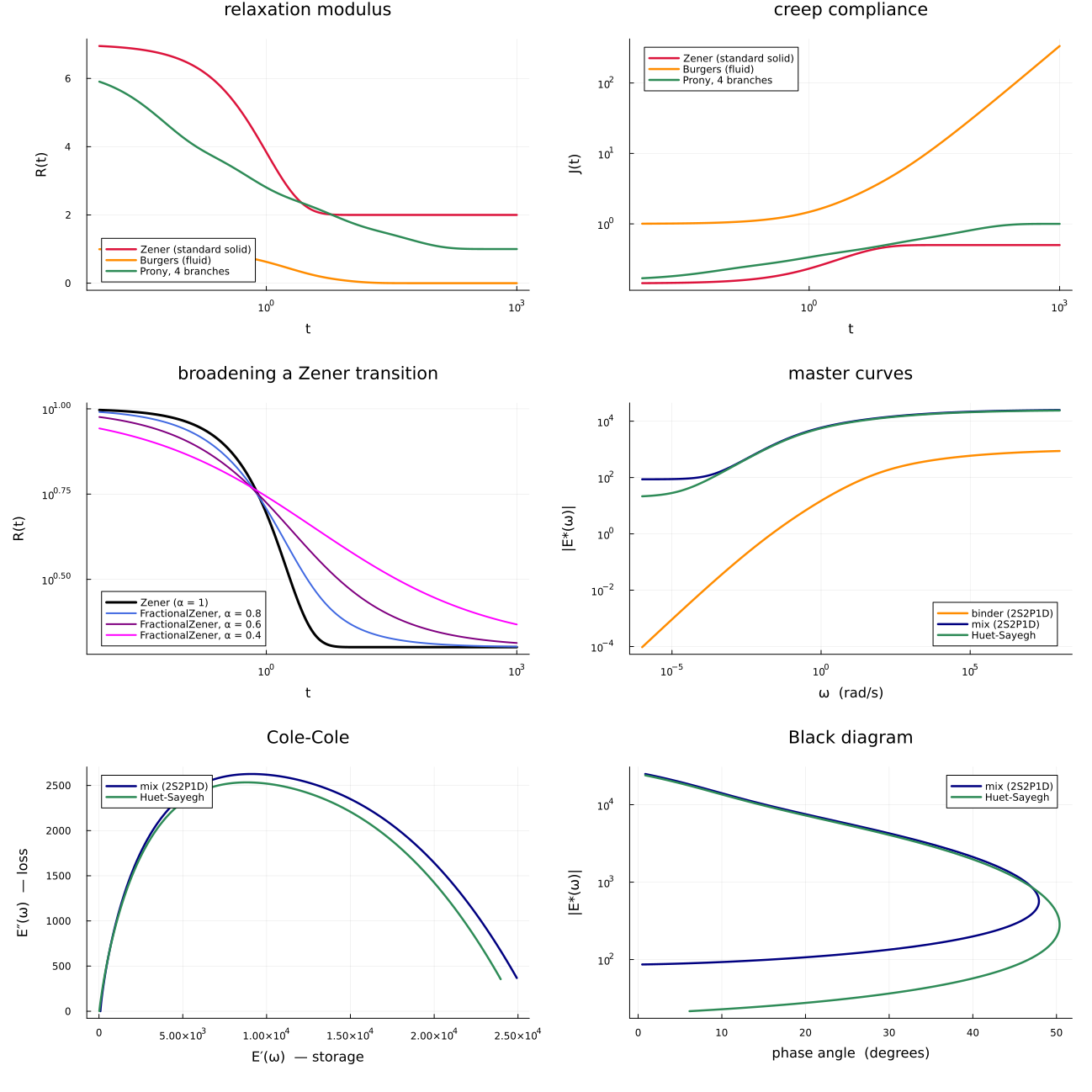

---

This page was generated using Literate.jl.