Ageing creep: loading age against inclusion shape

An ageing viscoelastic material is one whose creep compliance depends on the loading time and not only on the elapsed duration  . Concrete is the standard example: a specimen loaded at 40 days creeps less than the same specimen loaded at 1 day, because it has aged in the meantime.

This page runs one composite — a viscoelastic matrix with viscoelastic inclusions, 20 % by volume, homogenized by Mori-Tanaka — and sweeps the two parameters that fight each other:

• the loading age  , which is the ageing itself;

• the inclusion aspect ratio  , which is pure morphology and knows nothing about time.

Both act on the same output, the effective uniaxial creep function , and the point of the figure is how differently.

using MeanFieldHomogenization
using TensND
using LinearAlgebra
using Printf
using Plots
gr()

include(joinpath(pkgdir(MeanFieldHomogenization), "scripts", "common", "docviz.jl"))

_layer_colors (generic function with 1 method)

The microstructure

Spheroidal inclusions at 20 %, all aligned. Flattening them from   to   changes nothing about the phase properties — only how the matrix has to flow around them.

plotly_scene(
    rve_traces(; n = 60, semi_axes = (0.085, 0.085, 0.028), seed = 1949,
        orientation = (0.0, 0.0, 1.0));
    uid = "aa-rve", height = 470,
    title = "Aligned oblate inclusions, ω = 1/3 (drawn thicker than the run for legibility)"
)

Two ageing creep laws

Each phase creeps in two additive parts: a relaxing elastic term whose amplitude decays with the loading age — this is the ageing — and a logarithmic creep term in the elapsed duration  . Written on the spherical and deviatoric projectors and , a compliance is TensISO{3}(a, b) with the coefficient and the one.

# Matrix: E = 1, ν = 0.2.
const Es, νs = 1.0, 0.2
const ks, μs = k_mu(iso_stiffness_E_nu(Es, νs))
fk_s(tp) = 0.5 * exp(-tp / 20) + 0.5
fμ_s(tp) = 0.5 * exp(-tp / 20) + 0.5

function J_matrix(t, tp)
    a = fk_s(tp) / (3ks) + 1.0e-1 / ks * log(1 + (t - tp) / 2)
    b = fμ_s(tp) / (2μs) + 1.0e-1 / μs * log(1 + (t - tp) / 1)
    return TensISO{3}(a, b)
end

# Inclusions: stiffer and less compliant, E = 3, ν = 0.3, ageing faster.
const Ei, νi = 3.0, 0.3
const ki, μi = k_mu(iso_stiffness_E_nu(Ei, νi))
fk_i(tp) = 0.3 * exp(-tp / 10) + 0.4
fμ_i(tp) = 0.4 * exp(-tp / 15) + 0.3

function J_inclusion(t, tp)
    a = fk_i(tp) / (3ki) + 1.0e-1 / ki * log(1 + (t - tp) / 2)
    b = fμ_i(tp) / (2μi) + 1.0e-1 / μi * log(1 + (t - tp) / 1)
    return TensISO{3}(a, b)
end

const law_s = ViscoLaw(J_matrix, :creep)
const law_i = ViscoLaw(J_inclusion, :creep)

@printf "matrix    : k = %.4f  μ = %.4f\n" ks μs
@printf "inclusion : k = %.4f  μ = %.4f\n" ki μi

matrix    : k = 0.5556  μ = 0.4167
inclusion : k = 2.5000  μ = 1.1538

The time grid

A creep test loaded at needs a grid that starts at and resolves the first decade of the response, where the logarithmic term moves fastest. Two log-spaced stretches do that:   then  .

The grid is deliberately short (30 + 30 points): the ALV pipeline assembles and inverts a   Volterra matrix per run, so the cost grows as and this page performs eleven runs.

function creep_times(tp; n1 = 30, n2 = 30, tmax = 50.0)
    t0 = tp == 0 ? 1.0e-4 : float(tp)
    first_decade = exp10.(range(log10(t0), log10(t0 + 1); length = n1 + 1))[1:(end - 1)]
    tail = exp10.(range(log10(t0 + 1), log10(tmax); length = n2))
    return vcat(first_decade, tail)
end

creep_times (generic function with 1 method)

Uniaxial creep from the effective relaxation matrix

homogenize_alv returns the effective relaxation block matrix. Inverting it in the Volterra sense gives the creep matrix, and applying a unit uniaxial stress step at the first time of the grid gives the axial strain history — which is by definition.

function uniaxial_creep(R_eff, n)
    J_eff = volterra_inverse(R_eff; block_size = 6)
    Σ = zeros(6n)
    for i in 1:n
        Σ[6 * (i - 1) + 1] = 1.0            # unit axial stress, held constant
    end
    return (J_eff * Σ)[1:6:end]
end

function creep_composite(f, ω, times)
    r = RVE()
    add_phase!(r, :M, Spheroid(1.0), Dict(:C => law_s); fraction = :rest)
    add_phase!(r, :I, Spheroid(ω), Dict(:C => law_i); fraction = f)
    R = homogenize_alv(r, MoriTanaka(), :C; times = times)
    return uniaxial_creep(R, length(times))
end

# A single phase on its own needs no scheme: its own Volterra matrix is the
# answer, and going through an RVE of fraction 0 or 1 would only add a
# degenerate matrix phase.
function creep_single(law, times)
    J = trapezoidal_matrix(law, times)
    R = volterra_inverse(J; block_size = 6)
    return uniaxial_creep(R, length(times))
end

creep_single (generic function with 1 method)

The sweep

Three loading ages, three aspect ratios, plus the two pure phases as bounds.

const AGES = (0.0, 20.0, 40.0)
const OMEGAS = (1.0, 0.1, 0.01)
const F_INC = 0.2

results = Dict{Tuple{Float64, Any}, Tuple{Vector{Float64}, Vector{Float64}}}()
for tp in AGES
    times = creep_times(tp)
    results[(tp, :matrix)] = (times, Es .* creep_single(law_s, times))
    results[(tp, :inclusion)] = (times, Es .* creep_single(law_i, times))
    for ω in OMEGAS
        results[(tp, ω)] = (times, Es .* creep_composite(F_INC, ω, times))
    end
end

@printf "%-6s %-10s %10s %10s\n" "t'" "phase/ω" "J·E at t'+1" "J·E at 50"
for tp in AGES, key in (:matrix, OMEGAS..., :inclusion)
    t, J = results[(tp, key)]
    i1 = findfirst(≥(t[1] + 1 - 1.0e-9), t)
    @printf "%-6.0f %-10s %10.4f %10.4f\n" tp string(key) J[i1] J[end]
end

t'     phase/ω    J·E at t'+1  J·E at 50
0      matrix         1.1352     1.8246
0      1.0            0.8896     1.4507
0      0.1            0.7739     1.2895
0      0.01           0.7169     1.2142
0      inclusion      0.2788     0.5039
20     matrix         0.8192     1.3997
20     1.0            0.6341     1.1073
20     0.1            0.5409     0.9768
20     0.01           0.4933     0.9151
20     inclusion      0.1822     0.3721
40     matrix         0.7029     1.0588
40     1.0            0.5450     0.8356
40     0.1            0.4659     0.7344
40     0.01           0.4257     0.6858
40     inclusion      0.1582     0.2752

The table already shows the two effects separately. Reading down the blocks is ageing: the same microstructure loaded later creeps less. Reading across the three rows at fixed is morphology: flattening the inclusions makes the composite creep less. At equal volume fraction a flat stiff inclusion is the better reinforcement — the matrix cannot flow past it without straining it, so more of the load is carried by the phase that does not creep, and the effective compliance drops towards the inclusion bound.

The figure

One panel per loading age, so the ageing is the shift between panels and the shape effect is the spread inside each.

const COLORS = Dict(1.0 => :magenta, 0.1 => :red, 0.01 => :green)

panels = map(AGES) do tp
    p = plot(;
        xscale = :log10, xlabel = "t", ylabel = "E_mat · J_E^hom(t, t′)",
        title = "loading age t′ = $(Int(tp))", titlefontsize = 10,
        framestyle = :box, legend = (tp == AGES[1] ? :topleft : false),
        ylims = (0.0, 3.2)
    )
    t, J = results[(tp, :matrix)]
    plot!(p, t, J; lw = 2, color = :black, label = "matrix alone")
    t, J = results[(tp, :inclusion)]
    plot!(p, t, J; lw = 2, color = :blue, label = "inclusion alone")
    for ω in OMEGAS
        t, J = results[(tp, ω)]
        plot!(p, t, J; lw = 2, color = COLORS[ω], label = "f = $F_INC, ω = $ω")
    end
    p
end

p_all = plot(panels...; layout = (1, 3), size = (1080, 440),
    left_margin = 8Plots.mm, bottom_margin = 8Plots.mm, titlefontsize = 9)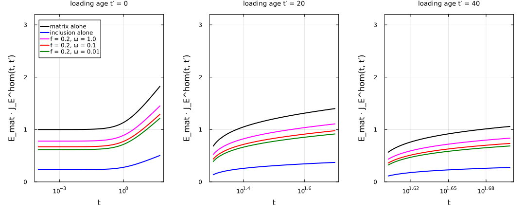

Three things are worth naming in that figure.

The composite is bracketed by its phases, at every time and every age. That is not automatic for an ageing problem — the bound holds here because both phases share the same kind of kernel.

Ageing shifts the whole family down. Between   and   the elastic amplitudes have decayed by roughly a factor of two, and the compliance at a fixed elapsed duration follows.

The aspect ratio orders the curves the same way at every age. Morphology and ageing do not interact here: the shape effect is a near-constant offset, which is exactly the property that makes it legitimate to calibrate a microstructure on one loading age and reuse it at another.

The shape effect, isolated

Dividing by the spherical case removes the ageing and leaves the morphology.

p_ratio = plot(;
    xscale = :log10, xlabel = "t − t′ + 1", ylabel = "J_E^hom(ω) / J_E^hom(ω = 1)",
    framestyle = :box, legend = :topleft, size = (760, 460),
    title = "Shape effect on the effective creep, f = $F_INC"
)
for tp in AGES, ω in (0.1, 0.01)
    t, J = results[(tp, ω)]
    _, J1 = results[(tp, 1.0)]
    plot!(p_ratio, t .- t[1] .+ 1, J ./ J1;
        lw = 2, color = COLORS[ω], ls = (tp == 0.0 ? :solid : tp == 20.0 ? :dash : :dot),
        label = "ω = $ω, t′ = $(Int(tp))")
end
p_ratio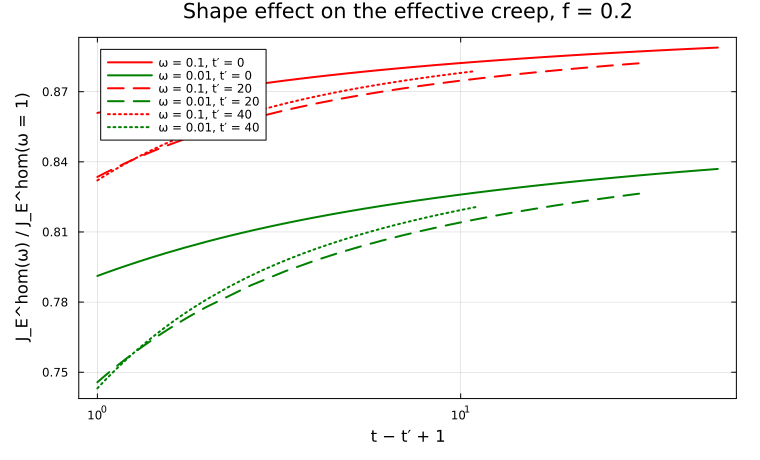

The three line styles are the three loading ages, and they nearly coincide: the ratio depends on and barely on . The morphological reduction of the creep — around 13 % at   and 19 % at  , at the end of the test — is a property of the shape alone.

for ω in (0.1, 0.01)
    line = String[]
    for tp in AGES
        _, J = results[(tp, ω)]
        _, J1 = results[(tp, 1.0)]
        push!(line, @sprintf("t′=%2.0f : %.4f", tp, J[end] / J1[end]))
    end
    @printf "ω = %-5s  %s\n" ω join(line, "   ")
end

ω = 0.1    t′= 0 : 0.8889   t′=20 : 0.8822   t′=40 : 0.8788
ω = 0.01   t′= 0 : 0.8370   t′=20 : 0.8264   t′=40 : 0.8206

See also

• Ageing viscoelastic schemes side by side — the same kind of test across Dilute / Mori-Tanaka / Maxwell / PCW

• Frequency or time? — when the non-ageing frequency route is enough

• Ageing creep of solidifying cementitious materials — an ageing model where the phase fractions also evolve

• The viscoelasticity manual — every ALV entry point

---

This page was generated using Literate.jl.