Homogenization schemes

MeanFieldHomogenization.Schemes computes the effective property tensor of a multi-phase medium from (i) the phase geometries, (ii) the phase properties and (iii) the phase volume fractions or crack densities.

Notation

The Representative Volume Element (RVE) consists of:

• a matrix phase of property tensor (or for the 2nd-order conductivity problem),

• one or more inclusion phases of property tensors , geometries , and amounts (volume fraction) or (crack density).

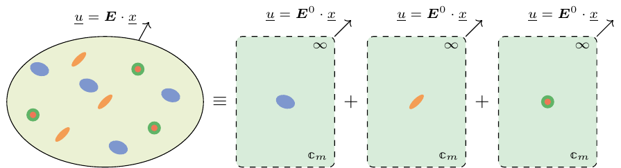
That picture is the mean-field approximation, and every scheme below is one answer to the single question it leaves open: what is , and in which medium is each inclusion embedded? Take   and the matrix as the reference and you have the dilute estimate; require the matrix average to come out right and you have Mori–Tanaka; embed each inclusion in the unknown effective medium and you have the self-consistent scheme.

For each inclusion the dilute strain concentration tensor and the size-independent stiffness contribution     are the natural building blocks ([24]). The dual compliance contribution     is more natural for cracks (whose stiffness contribution is the rank-1 limit of a divergent eigenvalue).

Bounds

Scheme	Formula
Voigt	(upper bound, [25])
Reuss	(lower bound)

Cracks are ignored in both bounds: their volume contribution vanishes in the penny limit ( ) while their density stays finite.

One-shot schemes (require a matrix)

Writing   for the total dilute stiffness contribution and  :

Scheme	Effective stiffness
Dilute	(first order in )
DiluteDual
Mori-Tanaka	([26], [27])
Maxwell	with the Hill tensor of the outer distribution shape
PCW	identical algebraic form, distribution-shape-aware ensemble interpretation ([28])

The second shape: Maxwell and PCW

Maxwell and PCW differ from the first three rows in that a second shape enters, describing how the inclusions are placed rather than what they look like. Maxwell reads it as one equivalent inclusion swallowing a cluster; PCW reads it as a safety ellipsoid around each inclusion:

Maxwell	Ponte Castañeda–Willis

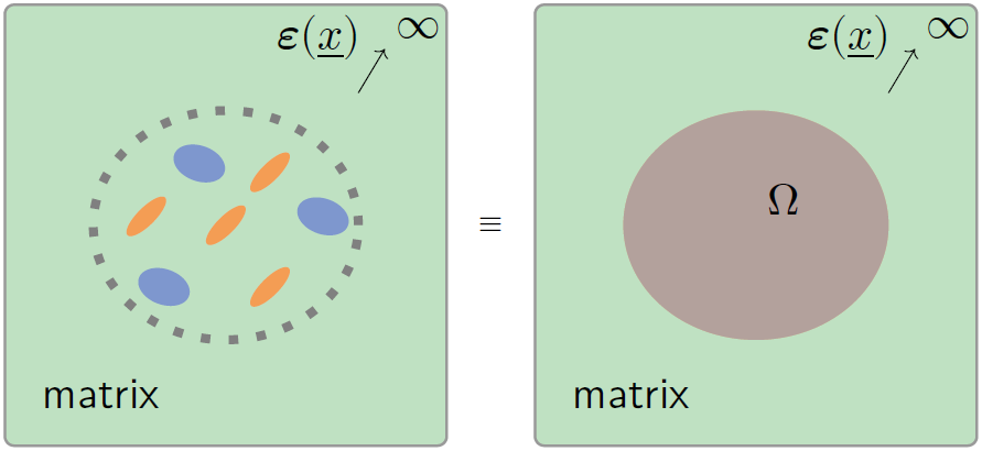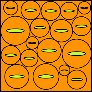The distribution shape is stored at the RVE level (default: unit sphere ⇒ Mori-Tanaka limit). Any AbstractInclusion can be used; the hierarchy AbstractDistributionShape leaves room for a future PairwiseDistribution extension following [29].

Iterative schemes

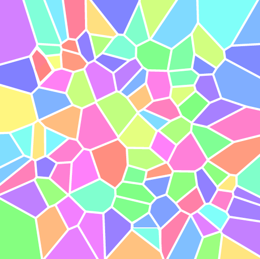
The one-shot schemes all need a phase to play the role of the matrix. When no phase does — a polycrystal, a granular assembly, a saturated foam — the reference medium has to be the effective medium itself, and the estimate becomes a fixed point:

Scheme	Iteration
SelfConsistent ([30])
AsymmetricSelfConsistent	switches between stiffness- and compliance-form iteration based on the matrix-vs-Voigt-bound contrast

The default solver is a damped Picard fixed point (Anderson with memory 1, Dual-safe). Loading NonlinearSolve.jl activates the MeanFieldHomogenizationNonlinearSolveExt extension, which accepts every SciML non-linear algorithm (NewtonRaphson(), TrustRegion(), Anderson(), …) via the algorithm keyword of SelfConsistent.

Differential scheme

The DifferentialScheme integrates the multi-phase incorporation ODE ([31]) on a fictitious incorporation time  ,

the increments following from the volume balance by Sherman-Morrison, along a user-selectable trajectory (Proportional, Sequential, CustomPath, Path). The dual form on the compliance is available through formulation = :compliance, and cracks — which have no volume but a finite density — enter with a balance of their own.

The trajectories agree in the dilute limit ( ) and diverge like at finite fractions — a physical feature of the scheme.

The full derivation, the crack case, the closed form of the homothetic trajectory and the SciML resolution are in The differential scheme.

N-body schemes (require positions)

Every scheme above — bounds, one-shot, iterative, differential — sees one inclusion in a reference medium and accounts for the others only through that reference: the interaction is treated in an average sense. Two schemes drop that one-site assumption and resolve the interaction inclusion by inclusion, which needs strictly more information than an RVE carries — the positions. They act on a ParticleAssembly instead, and share one ingredient, the two-inclusion interaction tensor .

Scheme	Unknowns	Reference
ClusterModel	mean strain of every family, from    — see the cluster model	[1]
EquivalentInclusion	polarization of every inclusion, from a Galerkin discretization of the weak Lippmann-Schwinger equation — see the equivalent inclusion method	[2]

The two are the same linear system on a periodic assembly and differ only in how the far field is closed. Both degenerate exactly onto Mori-Tanaka when the interaction is switched off — the sharpest available check that their assembly is right — and the equivalent inclusion method additionally returns a rigorous bound on the apparent stiffness.

Number-type compatibility

Every scheme is mandated to support:

• Float64 — default;

• ForwardDiff.Dual — sensitivity analysis through fractions, moduli, geometric parameters;

• Complex{Float64} — frequency-domain viscoelasticity (parity with the C++ ECHOES library, templated on T = double | complex<double>);

• SymPy.Sym, Symbolics.Num, BigFloat — best-effort, with explicit documentation of any limitation (the iterative SC solvers are not symbolic-friendly because the linear-system Jacobian must be numeric).