Crack opening displacement and compliance

A crack has no volume, so it cannot be described by a volume fraction and a stiffness. It is described instead by how much it opens under a given remote stress. That is the crack opening displacement tensor , and everything else on this page follows from it.

Read left to right: the COD tensor (order 2) gives the compliance contribution (order 4), which gives the dilute correction to the effective compliance; independently, gives the stress and displacement intensity factors , at the crack front.

MeanFieldHomogenization computes first — the intensity factors need it, and rebuilding from it avoids inverting a rank-deficient order-4 tensor. Its normalization is not unique in the literature, hence the Conventions section below.

Geometry

A flat crack is the limit of a flat spheroidal inclusion. Keeping the shape tensor of Notation,

with the in-plane unit vectors along the major and minor semi-axes  , and the unit normal.

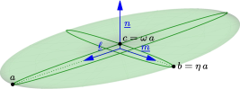
Two families matter, and they are genuinely different objects, not two regimes of one:

	geometry	in-plane aspect ratio	MeanFieldHomogenization type
elliptic (3-D)	bounded ellipse, semi-axes		EllipticCrack, PennyCrack for
ribbon (2-D)	infinite tunnel along , half-width	, so	RibbonCrack

The COD tensor

Under a remote stress , the two crack faces separate by the displacement jump . By linearity and the superposition principle, that jump depends on the loading only through the resolved traction   on the crack plane. Its average over the crack surface defines :

The normalization is by the in-plane half-width — the minor semi-axis of the ellipse, the half-width of the ribbon. This makes size-independent: it depends on the crack shape (through ) and on its orientation, never on how big it is. This is the convention of [42], following [43], [44], and it is the one MeanFieldHomogenization implements (cod_tensor, alias B_tensor).

The shape coefficient

The opening profile is an ellipsoidal cap, so the average jump is a fixed fraction of the maximum jump at the crack center:

is worth introducing explicitly, because every numerical factor on this page comes from it. It is the one quantity that distinguishes the elliptic geometry from the ribbon one.

The 3-D → 2-D limit: a trap

A ribbon is the limiting shape of an ellipse as  , so one expects to be . It is not [42]:

The reason is exactly . The geometry does converge, and so does the pointwise opening profile; what changes is the relation between the average opening and the maximum one, because averaging over a shrinking ellipse is not the same operation as averaging across the width of a strip ( ). Since is defined from the average, it picks up the ratio  .

This matters in practice: the intensity factors of an elliptic crack are computed from the ribbon tensor of the tangent ribbon at each front point (see Intensity factors at the crack front below), so both objects appear in the same formula and must not be confused.

From to the compliance

The extra strain a crack contributes, per unit volume of the embedding ellipsoid, is the average of the displacement jump over the crack surface , spread over the volume :

using the definition of . Identifying this with  , where      is the second Hill tensor, gives     , and hence

The limit is finite: the components diverge like , so   stays bounded. Evaluating the geometric factor for each family gives the two numbers used in the code:

	surface	volume
elliptic (3-D)
ribbon (2-D)

Both factors are independent of , which is the point of normalizing the limit by : one definition covers the 2-D and the 3-D geometry, and inherits 's size-independence.

The bridge in both directions is compliance_from_cod / cod_from_compliance (src/Cracks/cod_H_bridge.jl), dispatching on the crack type to apply the correct factor.

Conventions: what and are normalized by

The above looks like it disagrees with the literature. It does not — the three sources normalize the limit differently, while agreeing on . Naming them once avoids a great deal of confusion:

convention	elliptic	ribbon
MeanFieldHomogenization — limit normalized by , uniformly
Echoes and [45] — elliptic normalized by

So the two elliptic compliances differ by exactly :

They coincide for the penny crack  , which is why the discrepancy is invisible on the most common test case — and why a penny-only cross-check cannot detect a wrong -dependence.

Measured, not inferred from the papers — Echoes' crack_compliance against compliance_contribution on a flat triaxial ellipsoid ( ,  ,  ):

	1.0	0.7	0.5	0.3	0.1
	1.0000	0.7000	0.5000	0.3000	0.1000

On the MeanFieldHomogenization side the is -independent to machine precision (  for every ).

The COD tensor is the same, the compliance is not

All three sources normalize by the half-width , so the COD tensors agree. Only the compliance differs, and only for the elliptic crack. If you compare a across papers, expect agreement; if you compare an , check the normalization first.

Checking without going through

The closed forms of the next section give , and follows from it by the . Comparing to those closed forms would therefore verify nothing: it is the same formula read twice.

Read from right to left the boxed definition is a recipe: take a flat ellipsoid, compute , assemble     , invert, scale by the flatness  . That path never touches the crack machinery, so agreement with compliance_contribution is evidence rather than tautology:

using MeanFieldHomogenization, TensND, Plots
gr()  # headless backend; GKSwstype is set to "100" in make.jl

E, ν = 210.0, 0.3
C₀ = TensISO{3}(E / (1 - 2ν), E / (1 + ν))   # (3k, 2μ)

## ω-family of the definition, evaluated at finite flatness
function H_from_hill(a, b, ω, C₀)
    P = hill_tensor(Ellipsoid(a, b, ω * b), C₀)
    Q = C₀ - C₀ ⊡ P ⊡ C₀
    return ω * inv(Q)
end

relerr(A, B) =
    maximum(abs(A[i,j,k,l] - B[i,j,k,l]) for i in 1:3, j in 1:3, k in 1:3, l in 1:3) /
    maximum(abs(B[i,j,k,l]) for i in 1:3, j in 1:3, k in 1:3, l in 1:3)

ωs = exp10.(range(-1, -3; length = 9))
plt = plot(; xscale = :log10, yscale = :log10, legend = :topleft,
           xlabel = "flatness ω = c/b", ylabel = "relative error on ℍ")
for η in (1.0, 0.5, 0.3)
    crack = η == 1.0 ? PennyCrack(1.0) : EllipticCrack(1.0, η)
    H_ref = compliance_contribution(crack, C₀)
    plot!(plt, ωs, [relerr(H_from_hill(1.0, η, ω, C₀), H_ref) for ω in ωs];
          marker = :circle, label = "η = $η")
end
plot!(plt, ωs, ωs; linestyle = :dash, color = :black, label = "slope 1")
plt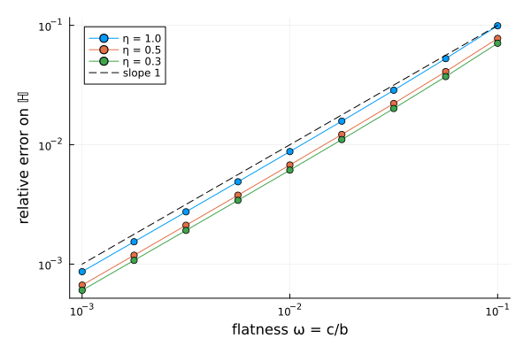

The three curves are straight lines of slope 1: the error decays like , which is the order of the Taylor term that resolves the limit ([46]). That slope is the real content of the check — a single would not distinguish a true limit from a coincidence.

Two limits of the flattening route

The Hill tensor is validated down to  , where the sweep stops, and the residue backend returns NaN below about   — hence method = :nestedquadgk for the anisotropic cases. Neither affects cod_tensor, which resolves the limit analytically instead of flattening an ellipsoid.

From the Green operator to

The closed forms of the next section are usually quoted. They are in fact derivable in closed form from the Fourier Green operator, and knowing where each factor comes from is what tells you which anisotropies admit a closed form at all. The script scripts/09_cod_symbolic_green.jl carries out the whole derivation symbolically, with the shipped closed forms as its oracles.

The reduced kernel

With     the acoustic (Christoffel) tensor, the two Fourier kernels of the traction integral equation on the crack plane are [47], [48]:

and the object the crack problem actually needs is the reduced transform — the Fourier transform of the restriction of to the crack plane [42]:

Two properties do all the work. Contracting twice with collapses the order-4 algebra to a 3×3 one,

which is the form every back-end evaluates (Core/green_helpers.jl). And is homogeneous of degree , so the singly contracted kernel decays like while the doubly contracted one decays like : the integral above converges as written, and is homogeneous of degree .

Three reductions, then the integral

The integrand is a rational function of whose denominator is , a sextic whose roots are the Stroh eigenvalues. Three structural reductions precede any integration:

1. Equivariance. When is invariant under rotations about — isotropic, or transversely isotropic with its axis along — so is the whole construction, since is also the integrated direction. One in-plane direction determines all of them.

2. Homogeneity. Degree factors out a single  .

3. Parity. The – block of the integrand is odd in and integrates to zero.

Together, with   and   :

For an isotropic matrix the sextic degenerates to  , leaving the single pair of double poles   , and the three coefficients are just the plane-strain and antiplane moduli:

For a transversely isotropic matrix with the crack in the plane of isotropy, every component , carries an odd number of indices and therefore vanishes: the antiplane (SH) polarization decouples, and the sextic splits into a quadratic and a biquadratic — solvable by radicals,

The radical of the published TI closed form ([49], [50]) is therefore nothing but the sum of the two in-plane Stroh roots — it comes out of the factorization rather than being postulated.

The crack-plane integral: where the elliptic integrals enter

On the crack contour     , so that  , and the of the degree-1 homogeneity cancels the of the two in-plane dyads. Exactly three angular integrals survive:

where, with    the Legendre parameter of Elliptic integrals,

the combinations stored by _elliptic_CS. The cross term vanishes by parity, which is why is diagonal in the crack frame.

Why cos² and sin² look exchanged against the literature

[42] defines the very same two quantities as

that is, over the complementary angle   , for which the radical above reads . Substituting swaps and in both the integrand and the radical, so the numbers are identical — verified to ten digits against the Legendre forms — while looks like a integral there and a integral here. Neither is wrong; only the origin of the angle differs. The above is the one to keep, because it is the angle the code integrates over (Cracks._cod_elliptic_numerical), matching the contour .

Hence

with the shape coefficient of the section above. The elliptic block is the same for the isotropic and the aligned-TI matrix — only change. That is why the two closed forms of the next section share one skeleton.

For the ribbon the contour integral is replaced by the single direction  , so   , and with  :

This is the exact identity behind the SIF ↔ DIF exchange relation at the end of this page: the operator that trades for is .

What breaks in the general case

Nothing above survives a general anisotropy: the acoustic tensor no longer block-decouples, is an irreducible sextic in , and the crack plane has no rotational symmetry left, so one in-plane direction no longer determines the others. Both integrals become numerical — which is what the Residue and cubature back-ends do, the first summing residues over the six Stroh roots located numerically.

Closed forms of

Isotropic matrix

For      with Young's modulus and Poisson ratio , in the crack frame :

with   and   the complete elliptic integrals of the first and second kind [13], provided by ell_K and ell_E.

The three components are the three fracture modes: opens the crack (mode I), and shear it (modes II and III).

Penny crack  , where   :

Implementation: src/Cracks/cod_analytical.jl, selected by method = :auto when is a TensISO{4,3}.

Transversely isotropic matrix

When the matrix is transversely isotropic with its axis aligned with the crack normal , is still analytical. The closed forms use the engineering parameters defined on the compliance   [49], [48], [50], and reduce to the isotropic case for   ,   . The auxiliary coefficients are documented inline in src/Cracks/cod_analytical.jl.

The more general cases — a TI axis not aligned with the crack normal, or an elliptic-orthotropic matrix — are treated in [45] and [42] but are not yet exposed here.

Arbitrary anisotropy — numerical

No closed form exists in general. Following [46], the limit   is resolved by extracting the first-order term of the Taylor expansion of in ; that term has an integral representation on the unit circle of the crack plane, evaluated by either algorithm trait:

• DECUHR — adaptive cubature [17], ForwardDiff-safe (src/Cracks/green_decuhr.jl);

• Residue — Cauchy-residue reduction to a 1-D quadrature, as in [16] adapted to the crack kernel, Float64 only (src/Cracks/green_residue.jl).

method = :auto always picks a cubature, never Residue: DECUHR when its weak dependency is loaded, and the type-generic NestedQuadGK otherwise — which is also what a ForwardDiff.Dual or symbolic scalar gets. Residue is faster but its acoustic polynomial degenerates when the reference is anisotropic in type and isotropic in value, a case the self-consistent and differential schemes reach at their first step, so it is available on explicit method = :residues only (src/Core/dispatch.jl).

Dilute correction to the effective compliance

compliance_contribution(crack, C₀) returns itself — the size-independent contribution, not the dilute correction. Cracks have no volume fraction, so the amount of cracking is measured by a Budiansky crack density [51], [44], and reintroduced by delta_compliance:

	density	dilute correction
elliptic (3-D)	(number per unit volume × major × minor²)
ribbon (2-D)	(number per unit area × half-width²)

Implementation: src/Cracks/compliance.jl, dispatching on the crack shape.

Intensity factors at the crack front

At a point of the crack front, with in-plane outer normal and tangent   , the asymptotic expansions of the jump and the traction read [52], [53], [54]:

is the displacement intensity factor (DIF) and the stress intensity factor (SIF), normalized so that the local energy release rate is simply    [55], [56].

The central result of the anisotropic theory [57], [47], [48] is that SIF and DIF are purely local and are exchanged by the COD tensor of the ribbon crack tangent to the real crack at the observation point:

This holds whatever the matrix anisotropy and whatever the remote loading — and it is why , with its factor, cannot be dispensed with even when studying elliptic cracks.

Elliptic crack

Parametrize the front by an angle :

with the in-plane semi-axis tensor and its pseudo-inverse. Then

where the dimensionless front factor is

Ribbon crack

Here    and  :

The SIF of an infinite ribbon crack is independent of the matrix stiffness — the of the DIF cancels against its inverse in the exchange relation.

Modes

Evaluation: sif and dif (src/Cracks/sif.jl).

Dispatch

(crack, C₀)	:auto selects	alternatives	ForwardDiff
EllipticCrack / RibbonCrack, TensISO	Analytical	—	✓
EllipticCrack / RibbonCrack, TensTI (aligned)	Analytical (MFH)	—	✓
EllipticCrack / RibbonCrack, AbstractTens{4,3}	DECUHR if loaded, else NestedQuadGK	:residues, :decuhr, :nestedquadgk	✓

Entry points: cod_tensor / B_tensor for , compliance_contribution for , delta_compliance for , sif / dif for the front quantities. The transport counterpart — a scalar COD and a rank-1 resistivity contribution — is treated in Thermal cracks, with the same geometric factors and .