Hill polarization tensors

The Eshelby problem reduces to computing one object, the Hill polarization tensor . This page gives its closed forms.

The structure to keep in mind: factors into a purely geometric part, which depends on the ellipsoid alone, and a purely material part, which depends on the reference moduli alone. The geometric part is a set of Newton-potential integrals; every shape — triaxial ellipsoid, spheroid, sphere, infinite cylinder — is one column of the same two tables.

This page follows the appendix Hill polarization tensors of the Echoes manual; expressions, conventions and bibliography are aligned on it. Extensions specific to MeanFieldHomogenization are flagged as such.

Those columns are the shapes below — meridian sections, drawn to scale from the semi-axes each closed form is written in. Every one of them is a limit of the same triaxial ellipsoid, reached by sending an aspect ratio to 1, 0 or ∞: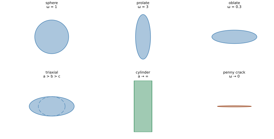

Two of the six are limits rather than bounded bodies: the cylinder leaves the panel because it is unbounded along its axis, and the penny crack is flat rather than thin. The dashed outline in the triaxial panel is the second principal section — the case where no two semi-axes coincide, and the only one that needs the general cubature.

The ribbon crack is deliberately absent: it is the   limit of the penny crack, so in a meridian section it draws exactly the same flat segment. What distinguishes it lies in the crack plane, which this view cannot show — hence the separate RibbonCrack type, and the   column of every table below.

The flat limits are the ones that need care: stays finite there, but the object built on it, , degenerates in a controlled way — which is why the crack theory is written on (Crack opening displacement).

Newton-potential integrals

Three integrals over the unit sphere, depending on only, factor every analytical Hill formula:

The two parametrizations of are related by the bijection of the unit sphere onto itself     , whose surface-element identity is

An intrinsic proof is given in [9], as an alternative to the component reasoning of [10]. Both forms are useful: the form makes the geometry explicit, the form is the one that degenerates cleanly in the cylinder limit below.

In MeanFieldHomogenization these are tens_IA, tens_UA and tens_VA.

Principal coefficients

and share their eigenvectors, so

The coefficients , identified with Newton-potential integrals [11], [6], [12], and the secondary coefficients admit closed forms in every symmetry class:

	ellipsoid	prolate spheroid	oblate spheroid	sphere	cylinder

Here   and   are the incomplete elliptic integrals of the first and second kind [13], of amplitude and parameter

The secondary coefficients follow from the by

except where the denominator degenerates — each symmetry class then has its own regular expression:

	ellipsoid	prolate spheroid	oblate spheroid	sphere	cylinder

with  . The circular cylinder   gives    and    .

Normalization differs from the classical references

For writing convenience the coefficients tabulated above are rescaled relative to [11] and [6]: they differ by a factor for with  , and by for all the others. The normalization used here is the one that makes  .

Internally, newton_potential_3d and newton_potential_3d_cylinder return the raw kernel — the values above multiplied by — and the division is applied at the tens_IA call site.

Why the cylinder column has zeros that still matter

The cylinder column is the limit   of the triaxial one. Three entries vanish, but they carry finite products that survive:

These products appear only through terms ( ) in , where they produce the vanishing first row and column of below and keep the third Eshelby identity valid at the cylinder endpoint. The circular sub-case   is evaluated on a separate branch, avoiding the   intermediates.

Identities

Always satisfied, and useful as numerical checks [6]:

Components of and

Both are orthotropic along the ellipsoid axes. In the principal frame [9], [5]:

Sphere  :

Infinite elliptic cylinder  , axis , transverse semi-axes   ([10], §11.22) — substituting the cylinder column above:

in Kelvin–Mandel storage and in the frame . The vanishing first row and column is the signature of the infinite cylinder: no polarization is transmitted along its axis. For the circular cylinder   the non-zero entries reduce to   ,  ,  , and to the diagonal .

Hill tensor in elasticity

Arbitrary anisotropy

[8], see also [10]. Inverting the acoustic tensor    pointwise is the source of all the computational work: in general no closed form exists and one resorts to numerical cubature [14], [15], [16]. MeanFieldHomogenization offers three algorithm traits, mirroring the Echoes NUMINT / RESIDUES options:

• DECUHR — the surface integral is evaluated by the adaptive cubature for singular integrands of [17]. ForwardDiff-safe. Selected by :auto when its (weak-dependency) extension is loaded.

• NestedQuadGK — nested adaptive 1-D quadrature, type-generic and always available; the :auto choice otherwise, and the one used for Dual, Complex and symbolic coefficients whatever else is loaded.

• Residue — the inner integral is reduced to a sum of residues by the Cauchy theorem, leaving a single 1-D quadrature [16]. The fastest of the three (~4 ms against ~11 ms and ~31 ms on a triaxial ellipsoid), but reachable on an explicit method = :residues only: it is Float64-only (the polynomial root finder it needs is not differentiable by ForwardDiff), and its acoustic polynomial degenerates when the reference is anisotropic in type while isotropic in value — returning NaN there instead of a number. That reference is what the differential and self-consistent schemes feed back at their first step, hence the choice of a cubature as the default.

Analytical paths exist in the literature for further anisotropy classes ([18], [19], [20], [21]) and are not all implemented yet.

Isotropic matrix — the shape/moduli factorization

With bulk modulus , shear modulus and first Lamé parameter   , so that         , the general expression collapses to [8]

This is the factorization announced at the top of the page: shape and orientation on one side (, ), reference moduli on the other. Each shape column of the tables above therefore yields a closed-form at once.

For a sphere, substituting and gives the classical Eshelby result

For an infinite cylinder, substituting and gives a closed form with  , i.e. no polarization along the axis ([10], §11.22).

Implementation: src/Elasticity/hill_3d_iso.jl and src/Elasticity/hill_3d_cylinder_iso.jl, selected by method = :auto when is a TensISO.

Transversely isotropic matrix coaxial with a spheroid

When the matrix is transversely isotropic and its symmetry axis is parallel to the spheroid axis, a fully analytical path exists [5]. The Hill tensor is transversely isotropic too, hence five Walpole coefficients (see Notation — there is no because is major-symmetric):

The five coefficients are closed-form combinations of acosh and complex square roots (equations 53–58 of [5]), depending on the aspect ratio (axial / transverse) and the five independent constants .

The dispatcher routes a TensTI{4} matrix combined with a coaxial Ellipsoid{3, Spherical|Prolate|Oblate} to this path by default; coaxiality is detected by _ti_coaxial(C₀, ell). Non-coaxial spheroids and triaxial ellipsoids fall back to the anisotropic default, i.e. a cubature. Implementation: src/Elasticity/hill_3d_ti_coaxial.jl.

Anisotropic matrix, cylinder limit

Cylinder is a first-class inclusion type here (extension over Echoes). For an arbitrarily anisotropic matrix the residue algorithm does not apply: it rests on the six complex roots of the acoustic polynomial along , and at the cylinder limit one root escapes to infinity, degenerating the polynomial.

The form of the Willis integral degenerates cleanly instead. The axial component of vanishes identically, so the surface integral collapses to a single quadrature over the transverse unit circle:

This is a one-dimensional QuadGK integral, and it stays ForwardDiff-compatible. Calling hill_tensor(Cylinder(…), C₀; method = :residues) falls back to it silently. Implementation: src/Elasticity/hill_3d_cylinder_aniso.jl (CylinderQuadrature trait). The in-plane components coincide with the solution of the 2-D plane-strain problem — the cylinder is the 3-D realization of the 2-D ellipse.

2-D plane strain

Plane strain is handled directly (extension over Echoes), integrating over the unit circle   with a prefactor in place of . The isotropic case is analytical; the anisotropic one uses the residue reduction on the line integral.

Hill tensor in conductivity

Arbitrary anisotropy — closed form

For a conductivity tensor [8]:

Unlike the order-4 case, this integral has a closed form for any matrix anisotropy. Since is symmetric positive definite it has a square root,    , and the denominator can be absorbed into the change of variable    , which turns the anisotropic problem into an isotropic one for a fictitious ellipsoid of shape tensor  :

This is the transformation derivation of [22]; an equivalent Green's-function derivation is given in [23]. Since   need not be symmetric, the fictitious semi-axes and principal directions are obtained by diagonalizing    .

Isotropic matrix — immediate

If    the prefactor comes straight out:

For a sphere,   gives   and   — independent of . Implementation: src/Conductivity/hill_order2_3d.jl.

Dispatch

Entry point hill_tensor; shape tensor via shape_tensor; geometric auxiliaries via tens_IA, tens_UA, tens_VA.

(inclusion, C₀)	:auto selects	alternatives	ForwardDiff
Ellipsoid{3}, TensISO	Analytical	—	✓
Ellipsoid{3}, TensTI (coaxial)	Analytical (MFH)	:residues, :decuhr	✓
Ellipsoid{3}, AbstractTens{4,3}	DECUHR if loaded, else NestedQuadGK	:residues, :decuhr, :nestedquadgk	✓
Cylinder, TensISO	Analytical	—	✓
Cylinder, AbstractTens{4,3}	CylinderQuadrature	(residue degenerates)	✓
Ellipsoid{2}, TensISO	Analytical	—	✓
Ellipsoid{2}, AbstractTens{4,2}	Analytical (residue)	—	(Float64)
Ellipsoid{3}, AbstractTens{2,3}	Analytical ()	—	✓
Cylinder, AbstractTens{2,3}	Analytical	—	✓

Cylinder shape traits: CircularCylindrical when   (transversely isotropic response, returned as TensTI{4} with axis ) and EllipticCylindrical when   (orthotropic, returned as TensOrtho). Practical usage is covered in the manual page Cylindrical inclusions.