Cement paste: chloride diffusivity and elasticity

Following [83] — and mirroring the corresponding chapter of the Echoes book [73] — this page builds a multi-scale micromechanical model of Portland cement paste that simultaneously predicts its elastic moduli and its chloride diffusivity from a single microstructural description, as a function of the water-to-cement ratio and the hydration degree .

Two models of increasing complexity are presented:

• an engineering model (two scales): hydrate foam + clinker;

• a detailed model (three scales): C-S-H gel → hydrate layers → cement paste.

The self-consistent scheme is used at each scale to capture the percolation of both the solid skeleton (governing stiffness) and the pore network (governing diffusivity). The detailed model assembles a genuine composite sphere — an anhydrous core coated by inner- and outer-hydrate shells — which enters the scheme through its concentration tensors, exactly as in [73].

Because a single RVE carries several property keys at once, the same microstructure is homogenized for stiffness (:C, a 4th-order tensor) and for diffusivity (:D, a 2nd-order tensor). All diffusivities are normalized by the bulk-water value  .

using MeanFieldHomogenization
using TensND
using LinearAlgebra
using Plots
gr()  # headless backend; GKSwstype is set to "100" in make.jl

# Isotropic property helpers.
Diso(d) = TensISO{3}(d)             # isotropic 2nd-order diffusivity d·𝟏
avg_D(D) = tr(Array(D)) / 3         # scalar diffusivity from a 2nd-order tensor
const D_bulk = Diso(1.0)            # capillary / bulk-water diffusivity
const Z4 = TensISO{3}(0.0, 0.0)     # empty pore stiffness
const Z2 = Diso(0.0)                # zero diffusivity (impervious solid)

Volume fractions: Powers' hydration model

The volume fractions of the main phases follow Powers' hydration model as functions of and [83]:

with   (clinker-to-water density ratio) and   (hydrate volume per unit volume of clinker). Hydration stops when the pore space is filled:

The Tennis–Jennings correlation [80] gives the mass ratio of low-density (LD) to total C-S-H, which splits the hydration products into an inner layer (HD-C-S-H, porosity  ) and an outer layer (LD-C-S-H,  ), with a fraction   of crystalline hydrates (portlandite) in each.

const ρ_a, κ_h, η = 3.13, 2.13, 0.20
const φ_HD, φ_LD = 0.24, 0.37
const φ_od0 = 0.63          # initial small-capillary fraction in the outer domain

αmax(wc) = min(1.0, wc * ρ_a / (κ_h - 1.0))

fa(wc, α) = (1.0 - α) / (1.0 + ρ_a * wc)
fh(wc, α) = κ_h * α / (1.0 + ρ_a * wc)
fcp(wc, α) = max(0.0, 1.0 - fa(wc, α) - fh(wc, α))

mLD(wc, α) = min(1.0, 0.538 + α * (3.017wc - 1.347))
function μLD(wc, α)
    mr = mLD(wc, α)
    return mr * (1.0 - φ_HD) / (1.0 - φ_LD + mr * (φ_LD - φ_HD))
end

fihp(wc, α) = (1.0 - μLD(wc, α)) * fh(wc, α)   # inner hydration products
fohp(wc, α) = μLD(wc, α) * fh(wc, α)           # outer hydration products

function ψf(wc, α)
    denom = 1.0 - fa(wc, α) - fihp(wc, α)
    return denom < 1.0e-12 ? 0.0 : fohp(wc, α) / denom
end
function fscp(wc, α)                            # small capillary pores
    φ = φ_od0 * (1.0 - ψf(wc, α))
    return fohp(wc, α) * φ / max(1.0 - φ, 1.0e-12)
end
flcp(wc, α) = max(0.0, fcp(wc, α) - fscp(wc, α))  # large capillary pores

(fa = round(fa(0.4, 0.8), digits = 4), fcp = round(fcp(0.4, 0.8), digits = 4))

(fa = 0.0888, fcp = 0.1545)

Engineering model

The engineering model [72, 83] involves two homogenization steps:

1. Level I — hydrate foam (self-consistent): an aging disordered assemblage of hydration products and capillary pores. The hydrates are oblate spheroids ( ) so that the solid percolates at the observed setting degree; the capillary pores are prolate ( ) so the pore network stays connected throughout hydration.

2. Level II — cement paste (Mori-Tanaka): spherical anhydrous clinker inclusions embedded in the hydrate-foam matrix.

The same phase properties serve the mechanical and the diffusion problems.

const C_anhyd = iso_stiffness_E_nu(135.0, 0.3)    # anhydrous clinker
const C_hyd = iso_stiffness_E_nu(25.3, 0.29)      # hydration products (calibrated)
const D_hyd = Diso(5.04e-4)                       # hydrate diffusivity (Yu 1991 fit)

const ω_h, ω_cp = 0.013, 6.0

function engineering_model(wc, α = -1.0)
    α < 0 && (α = αmax(wc))
    _fa, _fh, _fcp = fa(wc, α), fh(wc, α), fcp(wc, α)
    ft = _fh + _fcp                       # foam total (= 1 - fa)
    ft < 1.0e-10 && return (nothing, nothing)

    # Level I — hydrate foam (SC): HYD taken as the reference matrix.
    foam = RVE()
    add_phase!(foam, :HYD, Ellipsoid(1.0, 1.0, ω_h), Dict(:C => C_hyd, :D => D_hyd); fraction = :rest, symmetrize = IsoSymmetrize())
    add_phase!(
        foam, :CAP, Ellipsoid(1.0, 1.0, ω_cp), Dict(:C => Z4, :D => D_bulk);
        fraction = _fcp / ft, symmetrize = IsoSymmetrize()
    )
    C_foam = homogenize(foam, SelfConsistent(), :C)
    D_foam = homogenize(foam, SelfConsistent(), :D)

    # Level II — cement paste (MT): clinker spheres in the foam matrix.  The
    # diffusion step stays meaningful even before the solid skeleton percolates
    # (the impervious clinker still dilutes the foam diffusivity), so it is
    # computed unconditionally; only the stiffness is gated on percolation — as
    # in the Echoes reference, whose `C_foam.k` returns NaN below the threshold
    # and thus falls through to the same clinker-diluted diffusion.
    paste = RVE()
    add_phase!(paste, :FOAM, Ellipsoid(1.0, 1.0, 1.0), Dict(:C => C_foam, :D => D_foam); fraction = :rest)
    add_phase!(
        paste, :CLINKER, Ellipsoid(1.0, 1.0, 1.0), Dict(:C => C_anhyd, :D => Z2);
        fraction = _fa
    )
    D_cp = homogenize(paste, MoriTanaka(), :D)
    k_mu(C_foam)[1] < 1.0e-6 && return (0.0, avg_D(D_cp))  # foam not percolated ⇒ E=0

    C_cp = homogenize(paste, MoriTanaka(), :C)
    return (E_nu(C_cp)[1], avg_D(D_cp))
end

engineering_model(0.4, 0.6)

(13.955316732214074, 0.004617955939166672)

One microstructure, two physics

The two-scale chain above homogenizes the same foam twice — once for :C and once for :D — and then hands both results to the paste. Written declaratively, the foam is described once and the same nested object answers both keys, because a Homogenized with no explicit property inherits the key it is stored under:

function engineering_declarative(wc, α = -1.0)
    α < 0 && (α = αmax(wc))
    _fa, _fh, _fcp = fa(wc, α), fh(wc, α), fcp(wc, α)
    ft = _fh + _fcp

    foam = RVE()
    add_phase!(foam, :HYD, Ellipsoid(1.0, 1.0, ω_h), Dict(:C => C_hyd, :D => D_hyd); fraction = :rest, symmetrize = IsoSymmetrize())
    add_phase!(foam, :CAP, Ellipsoid(1.0, 1.0, ω_cp), Dict(:C => Z4, :D => D_bulk);
        fraction = _fcp / ft, symmetrize = IsoSymmetrize())

    h = Homogenized(foam, SelfConsistent())          # answers :C AND :D
    paste = RVE()
    add_phase!(paste, :FOAM, Ellipsoid(1.0, 1.0, 1.0), Dict(:C => h, :D => h); fraction = :rest)
    add_phase!(paste, :CLINKER, Ellipsoid(1.0, 1.0, 1.0),
        Dict(:C => C_anhyd, :D => Z2); fraction = _fa)
    return paste
end

let wc = 0.4, α = 0.6
    paste = engineering_declarative(wc, α)
    E_d = E_nu(homogenize(paste, MoriTanaka(), :C))[1]
    D_d = avg_D(homogenize(paste, MoriTanaka(), :D))
    E_x, D_x = engineering_model(wc, α)
    (ΔE = abs(E_d - E_x), ΔD = abs(D_d - D_x))
end

(ΔE = 0.0, ΔD = 0.0)

The two agree exactly. Note what the declarative form does not change: the percolation gate (k_mu(C_foam)[1] < 1e-6 ⇒ E = 0) is a decision taken between the scales, so it stays in the explicit driver — which is why the production model on this page keeps the explicit form. The declarative variant is shown here for the microstructure-description saving, which is what it is good at.

The effective Young's modulus and (log-scale) chloride diffusivity over the whole hydration range, for a set of water-to-cement ratios:

const WC_LIST = (0.30, 0.40, 0.50, 0.60)

function model_curves(model, wc; n = 60)
    # Linear α grid, as in the Echoes reference (from α = 0.02 to α_max).
    αs = range(0.02, αmax(wc); length = n)
    E = Float64[]
    D = Float64[]
    a = Float64[]
    for α in αs
        e, d = model(wc, α)
        (e === nothing || d === nothing) && continue
        push!(a, α); push!(E, e); push!(D, d)
    end
    return a, E, D
end

function plot_model(model, title)
    pE = plot(; xlabel = "α", ylabel = "E_hom (GPa)", title = "$title — modulus",
        legend = :topleft, framestyle = :box)
    pD = plot(; xlabel = "α", ylabel = "D_hom / D_bulk", yscale = :log10,
        title = "$title — diffusivity", legend = :topright, framestyle = :box)
    for wc in WC_LIST
        a, E, D = model_curves(model, wc)
        plot!(pE, a, E; label = "w/c=$wc", lw = 2)
        plot!(pD, a, max.(D, 1.0e-8); label = "w/c=$wc", lw = 2)
    end
    return plot(pE, pD; layout = (1, 2), left_margin = 8Plots.mm, bottom_margin = 8Plots.mm, size = (1000, 450))
end

plot_model(engineering_model, "Engineering model")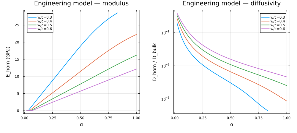

Detailed model

The detailed three-scale model tracks the C-S-H gel microstructure at the nanometer scale, the inner/outer hydrate layers at the micrometer scale, and the cement-paste assembly at the grain scale.

Level 0 — C-S-H gels

Both HD- and LD-C-S-H gels are self-consistent assemblages of oblate solid bricks ( ,   GPa,  , impervious) and prolate gel pores (  ,   ). The prolate pore shape is what keeps the gel diffusivity non-zero at the HD porosity  . The gel properties are fixed (independent of and ), so they are computed once.

const ω_s = 0.12
const ω_p = 1.0 / ω_s
const C_brick = iso_stiffness_E_nu(63.0, 0.27)
const C_crystal = iso_stiffness_E_nu(42.3, 0.324)   # portlandite
const D_gel = Diso(0.025)

function homogenize_csh(φ)
    gel = RVE()
    add_phase!(gel, :BRICK, Ellipsoid(1.0, 1.0, ω_s), Dict(:C => C_brick, :D => Z2); fraction = :rest, symmetrize = IsoSymmetrize())
    add_phase!(
        gel, :PORE, Ellipsoid(1.0, 1.0, ω_p), Dict(:C => Z4, :D => D_gel);
        fraction = φ, symmetrize = IsoSymmetrize()
    )
    C = homogenize(gel, SelfConsistent(), :C)
    D = homogenize(gel, SelfConsistent(), :D)
    return C, D
end

C_HD, D_HD = homogenize_csh(φ_HD)
C_LD, D_LD = homogenize_csh(φ_LD)
(E_HD = round(E_nu(C_HD)[1], digits = 2), D_HD = round(avg_D(D_HD), sigdigits = 3),
    E_LD = round(E_nu(C_LD)[1], digits = 2), D_LD = round(avg_D(D_LD), sigdigits = 3))

(E_HD = 31.04, D_HD = 0.000443, E_LD = 17.59, D_LD = 0.0016)

Level I — inner and outer hydrate layers

The inner layer is a self-consistent mixture of HD-C-S-H gel and spherical nano-crystals. The outer layer is built in two SC steps: oblate LD-C-S-H foam ( , the aspect ratio that controls its setting threshold) mixed with spherical small capillary pores, then folded together with spherical micro-crystals.

const ω_LD = 0.14

function inner_layer_props()
    r = RVE()
    add_phase!(r, :CSH, Ellipsoid(1.0, 1.0, 1.0), Dict(:C => C_HD, :D => D_HD); fraction = :rest)
    add_phase!(
        r, :CRYSTAL, Ellipsoid(1.0, 1.0, 1.0), Dict(:C => C_crystal, :D => Z2);
        fraction = η
    )
    return homogenize(r, SelfConsistent(), :C), homogenize(r, SelfConsistent(), :D)
end

const C_inner, D_inner = inner_layer_props()   # fixed, α-independent

function outer_layer_props(wc, α)
    _fohp, _fscp = fohp(wc, α), fscp(wc, α)
    f_ld = (1.0 - η) * _fohp
    f_tot = f_ld + _fscp
    f_tot < 1.0e-12 && return C_LD, D_LD
    φ_scp = _fscp / f_tot

    # Step 1 — oblate LD-C-S-H foam + spherical small capillary pores.
    r1 = RVE()
    add_phase!(r1, :LDCSH, Ellipsoid(1.0, 1.0, ω_LD), Dict(:C => C_LD, :D => D_LD); fraction = :rest, symmetrize = IsoSymmetrize())
    add_phase!(
        r1, :SCP, Ellipsoid(1.0, 1.0, 1.0), Dict(:C => Z4, :D => D_bulk);
        fraction = φ_scp
    )
    C1 = homogenize(r1, SelfConsistent(), :C)
    D1 = homogenize(r1, SelfConsistent(), :D)

    # Step 2 — outer C-S-H + spherical micro-crystals.
    η_out = η * _fohp / (_fohp + _fscp)
    r2 = RVE()
    add_phase!(r2, :CSH, Ellipsoid(1.0, 1.0, 1.0), Dict(:C => C1, :D => D1); fraction = :rest)
    add_phase!(
        r2, :CRYSTAL, Ellipsoid(1.0, 1.0, 1.0), Dict(:C => C_crystal, :D => Z2);
        fraction = η_out
    )
    return homogenize(r2, SelfConsistent(), :C), homogenize(r2, SelfConsistent(), :D)
end

Level II — cement paste

The paste is a generalized self-consistent scheme with two inclusion types: a three-layer composite sphere (anhydrous core + inner layer + outer layer) and spherical large capillary pores. The layer radii are recovered from the cumulative layer volume fractions; because a LayeredSphere stores one property family, the stiffness and diffusivity problems each get their own sphere (same radii, different per-layer moduli).

# Ascending radii from layer volume fractions g₁,…,g_M (outer radius = 1).
function layer_radii(gs)
    c = cumsum(collect(gs))
    total = c[end]
    return ntuple(k -> (c[k] / total)^(1 / 3), length(gs))
end

# Coerce a homogenized isotropic result to a TensISO the sphere can store.
iso_C(C) = (k = k_mu(C); iso_stiffness(k[1], k[2]))
iso_D(D) = Diso(avg_D(D))

function detailed_model(wc, α = -1.0)
    α < 0 && (α = αmax(wc))
    _fa, _fihp, _fohp = fa(wc, α), fihp(wc, α), fohp(wc, α)
    _fscp, _flcp = fscp(wc, α), flcp(wc, α)
    g = (_fa, _fihp, _fohp + _fscp)         # core, inner, outer
    f_layers = sum(g)
    f_layers < 1.0e-10 && return (nothing, nothing)
    g[1] < 1.0e-10 && return (nothing, nothing)   # no anhydrous core

    C_outer, D_outer = outer_layer_props(wc, α)
    radii = layer_radii(g)

    sphere_C = LayeredSphere(radii, (C_anhyd, iso_C(C_inner), iso_C(C_outer)))
    sphere_D = LayeredSphere(radii, (Z2, iso_D(D_inner), iso_D(D_outer)))

    rC = RVE()
    add_phase!(rC, :PASTE, Ellipsoid(1.0, 1.0, 1.0), Dict(:C => C_LD); fraction = :rest)   # SC: reference only
    add_phase!(rC, :LAYERS, sphere_C, Dict(:C => C_anhyd); fraction = f_layers)
    add_phase!(rC, :LCP, Ellipsoid(1.0, 1.0, 1.0), Dict(:C => Z4); fraction = _flcp)
    C_cp = homogenize(rC, SelfConsistent(), :C)

    rD = RVE()
    add_phase!(rD, :PASTE, Ellipsoid(1.0, 1.0, 1.0), Dict(:D => D_LD); fraction = :rest)
    add_phase!(rD, :LAYERS, sphere_D, Dict(:D => D_bulk); fraction = f_layers)
    add_phase!(rD, :LCP, Ellipsoid(1.0, 1.0, 1.0), Dict(:D => D_bulk); fraction = _flcp)
    D_cp = homogenize(rD, SelfConsistent(), :D)

    return (E_nu(C_cp)[1], avg_D(D_cp))
end

detailed_model(0.4, 0.6)

(13.382003926144565, 0.005398151121986632)

plot_model(detailed_model, "Detailed model")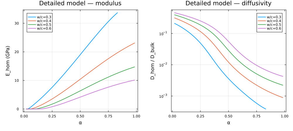

Comparison of both models

Both predict, for a given , a percolation threshold in stiffness near the observed setting degree and a sharp drop in diffusivity at intermediate-to-high hydration, as the large capillary pores disconnect and transport is forced through the poorly-diffusive gel. The engineering model is faster but calibrated on mature paste; the detailed one follows experiment more closely across the full hydration range [83].

wc = 0.4
ae, Ee, De = model_curves(engineering_model, wc)
ad, Ed, Dd = model_curves(detailed_model, wc)

pE = plot(; xlabel = "α", ylabel = "E_hom (GPa)", title = "Young's modulus — w/c=$wc",
    legend = :topleft, framestyle = :box)
plot!(pE, ae, Ee; label = "engineering", lw = 2, ls = :dash)
plot!(pE, ad, Ed; label = "detailed", lw = 2)

pD = plot(; xlabel = "α", ylabel = "D_hom / D_bulk", yscale = :log10,
    title = "Chloride diffusivity — w/c=$wc", legend = :topright, framestyle = :box)
plot!(pD, ae, max.(De, 1.0e-8); label = "engineering", lw = 2, ls = :dash)
plot!(pD, ad, max.(Dd, 1.0e-8); label = "detailed", lw = 2)

plot(pE, pD; layout = (1, 2), left_margin = 8Plots.mm, bottom_margin = 8Plots.mm, size = (1000, 450))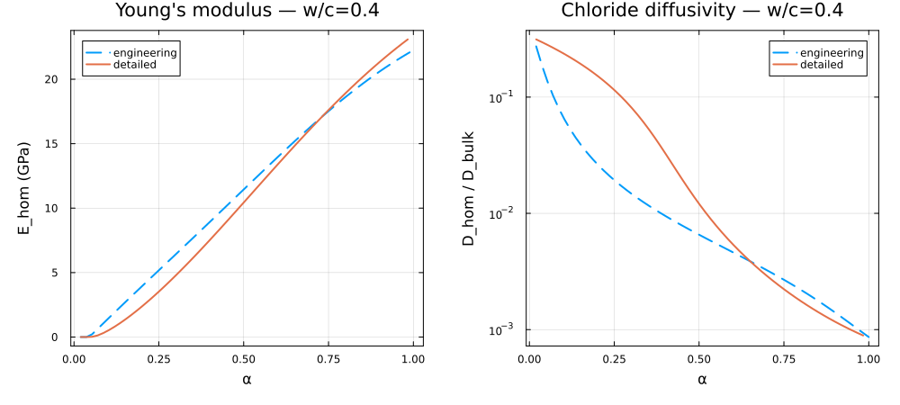

Percolation diagrams: role of the inclusion shapes

The oblate/prolate aspect ratios of the engineering model are not free: they are fixed by requiring the elastic and diffusion percolation thresholds to fall at the porosities observed experimentally [83]. For a self-consistent two-phase medium of solid spheroids (aspect ratio ,  , impervious) and pore spheroids (,  ,  ), both thresholds depend only on the two shapes, not on the (non-zero) modulus values.

The diffusion threshold — the porosity above which the pore network conducts — follows in closed form from the 2nd-order SC equation at  :

The elastic threshold — the porosity above which the solid skeleton loses rigidity,   — reduces to a coupled system in the solid fraction and the Poisson ratio of the SC medium, involving the Hill tensor   of the solid and the dual Hill tensor      of the pore (with the SC medium normalized to unit Young's modulus):

with   . These are exactly the relations of the Echoes book [73]; the two implementations agree to machine precision.

# Frobenius double-double contraction ⟨A,B⟩ = A_ijkl B_ijkl, matching the
# 6×6 Mandel `tr(A·B)` used in Echoes.
frob(A, B) = sum(Array(A) .* Array(B))
const 𝕁 = TensISO{3}(1.0, 0.0)
const 𝕂 = TensISO{3}(0.0, 1.0)

function bisect_root(f, lo, hi; n = 60)
    flo = f(lo)
    for _ in 1:n
        m = (lo + hi) / 2
        if flo * f(m) <= 0
            hi = m
        else
            lo = m; flo = f(lo)
        end
    end
    return (lo + hi) / 2
end

# Elastic percolation threshold φ_elas = 1 - f_s (pore fraction).
function φ_elas(ωs, ωp)
    Es, Ep = Ellipsoid(1.0, 1.0, ωs), Ellipsoid(1.0, 1.0, ωp)
    function invPQ(ν)
        C = iso_stiffness_E_nu(1.0, ν)
        iPs = inv(hill_tensor(Es, C))
        iQp = inv(C - C ⊡ hill_tensor(Ep, C) ⊡ C)   # dual Hill of the pore
        return iPs, iQp
    end
    solf(iPs, iQp, ν) = (a = frob(𝕁, iPs); b = frob(𝕁, iQp); b / ((1 - 2ν)^2 * a + b))
    function eqν(ν)
        iPs, iQp = invPQ(ν)
        f = solf(iPs, iQp, ν)
        return f * (1 + ν)^2 * frob(𝕂, iPs) - (1 - f) * frob(𝕂, iQp)
    end
    ν = bisect_root(eqν, 0.0, 0.4)
    iPs, iQp = invPQ(ν)
    return 1 - solf(iPs, iQp, ν)
end

# Diffusion percolation threshold (pore fraction) — closed form.
# `hill_tensor` returns a 2nd-order `Tens`; `tr`, `inv` and tensor subtraction
# are intrinsic TensND operations, so no array materialization is needed.
function φ_diff(ωs, ωp)
    Pp = hill_tensor(Ellipsoid(1.0, 1.0, ωp), TensISO{3}(1.0))
    Ps = hill_tensor(Ellipsoid(1.0, 1.0, ωs), TensISO{3}(1.0))
    a = tr(inv(Pp))
    b = tr(inv(TensISO{3}(1.0) - Ps))
    return b / (a + b)
end

(elastic = round(100 * φ_elas(0.013, 6.0), digits = 1),
    diffusion = round(100 * φ_diff(0.013, 6.0), digits = 1))

(elastic = 92.6, diffusion = 65.5)

The two thresholds, mapped over , with the calibration points of the engineering model () and of the C-S-H gel ():

n = 51   # same grid as Echoes (51×51 over log₁₀ω ∈ [−3, 2])
logω = range(-3.0, 2.0; length = n)
ω = 10.0 .^ logω
Ze = [100 * φ_elas(ω[i], ω[j]) for j in 1:n, i in 1:n]   # rows = ωp, cols = ωs
Zd = [100 * φ_diff(ω[i], ω[j]) for j in 1:n, i in 1:n]

cal_s = (log10(0.013), log10(0.12))
cal_p = (log10(6.0), log10(1 / 0.12))

function threshold_panel(Z, title)
    p = contour(logω, logω, Z; fill = true, c = :viridis, levels = 12,
        xlabel = "log₁₀ ωs (solid)", ylabel = "log₁₀ ωp (pore)",
        title = title, colorbar_title = " φ (%)", framestyle = :box)
    scatter!(p, [cal_s[1]], [cal_p[1]]; m = :star5, ms = 9, c = :red, label = "eng.")
    scatter!(p, [cal_s[2]], [cal_p[2]]; m = :utriangle, ms = 7, c = :white, label = "gel")
    return p
end

plot(threshold_panel(Ze, "Elastic φ_elas (%)"),
    threshold_panel(Zd, "Diffusion φ_diff (%)");
    layout = (1, 2), left_margin = 8Plots.mm, bottom_margin = 8Plots.mm, size = (1000, 450))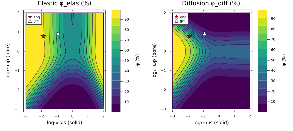

The same two threshold maps as interactive 3D surfaces over — rotate, zoom and hover to read values, exactly as the Echoes book renders them with Plotly:

# `plotly_surface` comes from the shared figure helpers — it emits a `<div>` plus
# a `<script>` that pulls plotly.js in *through* require.js, which is what
# Documenter pages need (see scripts/common/docviz.jl for why).
include(joinpath(pkgdir(MeanFieldHomogenization), "scripts", "common", "docviz.jl"))

plotly_surface(logω, logω, Ze; title = "Elastic percolation threshold φ_elas (%)",
    zlabel = "φ_elas (%)", uid = "surf-phi-elas",
    xlabel = "log₁₀ ωs", ylabel = "log₁₀ ωp", colorbar_title = "φ (%)")

plotly_surface(logω, logω, Zd; title = "Diffusion percolation threshold φ_diff (%)",
    zlabel = "φ_diff (%)", uid = "surf-phi-diff",
    xlabel = "log₁₀ ωs", ylabel = "log₁₀ ωp", colorbar_title = "φ (%)")

The thin oblate solid ( ) percolates at a tiny solid fraction, so the skeleton carries load up to   (early set, low ), while the prolate pores give   (late disconnection, high ): the two thresholds are well separated, which is what reproduces both the early set and the late diffusivity drop. The gel sits at   and  , so at   it is simultaneously load-bearing and diffusive — the prolate gel pores are what keep  .

Numerical agreement with Echoes

Evaluated with the compiled Echoes library, and at these points coincide with the values above to the third decimal (identical Poisson ratio at the elastic root), confirming that MeanFieldHomogenization and Echoes share the same Hill/dual-Hill kernels.