The rheological model library

A linear viscoelastic material is described by four equivalent functions — the relaxation modulus R(t), the creep compliance J(t), and their Laplace-Carson transforms R*(p) and J*(p). Which of them is elementary depends entirely on the model, so this library is built so that you never have to care: every model answers all four, whichever it was defined by.

using MeanFieldHomogenization

m = zener_maxwell(2.0, 5.0, 1.0)      # E_∞ = 2, one branch (E₁ = 5, τ₁ = 1)

(relaxation(m, 0.7), creep(m, 0.7), carson_relaxation(m, 0.7), carson_creep(m, 0.7))

(4.482926518957047, 0.2075961596150065, 4.0588235294117645, 0.24637681159420288)

1. The interface

Five generics cover every model, scalar or tensorial:

function	meaning
carson_relaxation(m, p)	— the only method a model must define
carson_creep(m, p)	; defaults to 1/carson_relaxation
relaxation(m, t)	; defaults to inverting
creep(m, t)	; defaults to inverting
complex_modulus(m, ω)

plus the limits glassy_modulus ( ) and equilibrium_modulus ( ), the predicate is_fluid, and the dynamic quantities storage_modulus, loss_modulus, loss_factor.

That fallback lattice is the design. Defining a new model means writing one method:

struct MyModel <: MeanFieldHomogenization.Viscoelasticity.AbstractRheology
    E::Float64
    τ::Float64
end

MeanFieldHomogenization.Viscoelasticity.carson_relaxation(m::MyModel, p) =
    m.E * (p * m.τ)^0.5 / (1 + (p * m.τ)^0.5)

creep(MyModel(10.0, 1.0), 2.0)        # obtained by numerical inversion

0.25957691216064194

Values obtained by inversion are accurate to about 1e-12 with the default method and are differentiable — see the inversion manual.

2. The catalog

Elementary elements

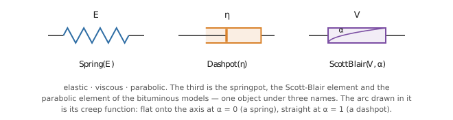
Spring(E)
Dashpot(η)
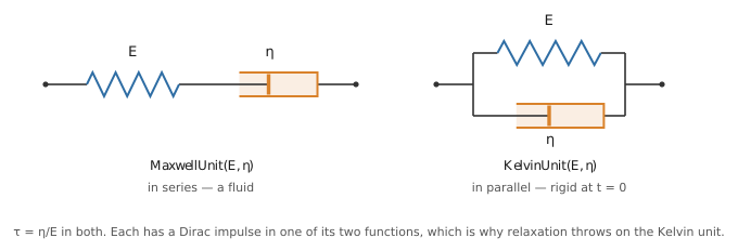
MaxwellUnit(E, η)
KelvinUnit(E, η)

with   in both cases. Dashpot and KelvinUnit have a Dirac impulse for a relaxation function, so relaxation and glassy_modulus throw on them rather than return a wrong number — assemble them with a spring first.

Discrete spectra

PronyRelaxation and PronyCreep are the workhorses:

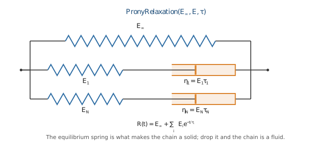
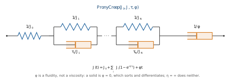
E_inf == 0 means a fluid; so does phi > 0 on the creep side. The two are converted into one another exactly by maxwell_to_kelvin and kelvin_to_maxwell — see the theory for why that is robust and the tutorial for what it looks like.

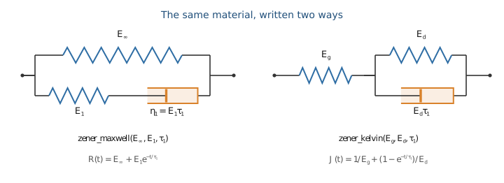
Named special cases: zener_maxwell and zener_kelvin (the standard linear solid, both ways round) and burgers.

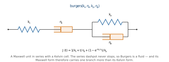
b = burgers(1.0, 3.0, 2.0, 6.0)       # k_s, η_s, k_p, η_p
r = kelvin_to_maxwell(b)
(is_fluid(b), length(r), equilibrium_modulus(r))   # a fluid gains one branch

(true, 2, 0.0)

Fractional elements

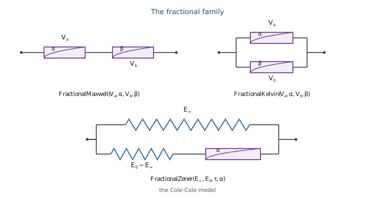
A single exponential spans one decade; real polymers and bitumen relax over six or more. The fractional elements broaden the spectrum without adding branches.

		notes
ScottBlair(V, α)		the springpot; α = 0 a spring, α = 1 a dashpot. All four functions closed form
FractionalMaxwell(V_a, α, V_b, β)	two springpots in series	a fluid
FractionalKelvin(V_a, α, V_b, β)		a solid when β = 0
FractionalZener(E_∞, E_0, τ, α)		the Cole-Cole model; is a Mittag-Leffler function
Rabotnov(μ₀, λ₀, α, β)		the ECHOES benchmark kernel

Rabotnov's transform is elementary

The kernel is usually written with a Mittag-Leffler function,    . Its Carson transform is simply  , which is what the table above shows — no special function is involved on this route at all. A passive material has  ; the benchmark of [59] §5 uses μ₀ = 1.7, λ₀ = -0.495, α = -0.46, β = 0.98.

The two models whose time-domain form is a Mittag-Leffler function use it when MittagLeffler.jl is loaded, and fall back on numerical inversion of the closed-form transform otherwise. Both routes agree to about 1e-10:

fz = FractionalZener(2.0, 10.0, 1.0, 0.6)
(relaxation(fz, 1.0), inverse_carson(p -> carson_relaxation(fz, p), 1.0))

(5.306618727549521, 5.306618727549521)

An upstream defect worth knowing about

MittagLeffler.jl v1.0.0 returns 1.0 for 1 < a < 2 and small |z|, silently — mittleff(1.3, 1.0, -0.5) gives 1.0 where the series gives 0.633. The extension therefore answers only for 0 < a ≤ 1, the domain checked against the series in the test suite; anything else falls back on the inversion, which is correct.

Bituminous binders and mixtures

HuetSayegh and Model2S2P1D are the reference models of the field:

with the bracketed series-dashpot term present in 2S2P1D and absent in Huet-Sayegh — which is exactly the difference between a fluid and a solid.

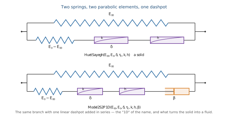
E00 is the static modulus and E0 the glassy one, following Di Benedetto and Olard and the ECHOES sources; 0 < k < h < 1.

2S2P1D is exact in both domains

Because   , the denominator is the transform of an ordinary function of time, term by term:

So the same object is an exact Laplace-Carson model and an exact Volterra model. creep_kernel gives , carson_creep_kernel gives , and creep_kernel_law packages the former as a ViscoLaw so that the ageing pipeline can consume it:

Φ = trapezoidal_matrix(creep_kernel_law(m), times)
R = m.E00 * I + (m.E0 - m.E00) * volterra_inverse(Φ; block_size = 1)

That discrete R must agree with relaxation(m, t) obtained by inverting the transform. It does, and that is the sharpest available check that the two routes of the package are consistent.

binder = Model2S2P1D(1.0e-7, 1000.0, 2.2, 1.94507827e-3, 0.22, 0.63, 50.0)
E = complex_modulus(binder, 2π * 10)          # 10 Hz
(abs(E), rad2deg(angle(E)))                   # norm and phase angle

(128.57911650285212, 35.2545015531917)

Long-term creep of concrete

LogarithmicCreep(E, C, τ) is    , whose transform involves the exponential integral,   . It is evaluated through SpecialFunctions.expintx, the scaled form, so it stays finite where alone would overflow.

The ageing version — where E, C and τ depend on the loading age — is a different object and belongs to the time-domain route.

3. Fitting a chain to something that is not one

When the material is given as an arbitrary transform — measured data, or a homogenized C*(p) — prony_fit_relaxation fits a discrete spectrum by collocation, and everything above becomes available:

fz2 = FractionalZener(2.0, 10.0, 1.0, 0.6)
fit = prony_fit_relaxation(p -> carson_relaxation(fz2, p), exp10.(range(-2, 2; length = 14)))
(count(>(0), fit.E), relaxation(fit, 1.0), relaxation(fz2, 1.0))

(7, 5.301066606139192, 5.306618727549521)

The fit is non-negative by default. That is what makes the result completely monotone and hence passive — and it also fits better: the unconstrained least-squares solution puts half its moduli below zero and is three times worse on the master curve.

A fit is a calibration step, not a differentiable one

With nonneg = true the solve is an active-set method, so the coefficients are a piecewise-smooth function of the input with a combinatorial switch in the middle. Differentiate the resulting model, not the fit. An unconstrained fit (nonneg = false) is a plain linear solve and is differentiable.

4. Lifting to a fourth-order tensor

iso_rheology pairs two scalar models into an isotropic tensor model, one per channel:

iso = iso_rheology(Spring(2500.0), binder)    # elastic bulk, 2S2P1D shear
carson_relaxation(iso, im * 2π * 10)

3×3×3×3 TensND.TensISO{4, 3, ComplexF64, 2}:
[:, :, 1, 1] =
 2640.0+98.9561im     0.0+0.0im        0.0+0.0im
    0.0+0.0im      2430.0-49.478im     0.0+0.0im
    0.0+0.0im         0.0+0.0im     2430.0-49.478im

[:, :, 2, 1] =
     0.0+0.0im      104.997+74.2171im  0.0+0.0im
 104.997+74.2171im      0.0+0.0im      0.0+0.0im
     0.0+0.0im          0.0+0.0im      0.0+0.0im

[:, :, 3, 1] =
     0.0+0.0im      0.0+0.0im  104.997+74.2171im
     0.0+0.0im      0.0+0.0im      0.0+0.0im
 104.997+74.2171im  0.0+0.0im      0.0+0.0im

[:, :, 1, 2] =
     0.0+0.0im      104.997+74.2171im  0.0+0.0im
 104.997+74.2171im      0.0+0.0im      0.0+0.0im
     0.0+0.0im          0.0+0.0im      0.0+0.0im

[:, :, 2, 2] =
 2430.0-49.478im     0.0+0.0im         0.0+0.0im
    0.0+0.0im     2640.0+98.9561im     0.0+0.0im
    0.0+0.0im        0.0+0.0im      2430.0-49.478im

[:, :, 3, 2] =
 0.0+0.0im      0.0+0.0im          0.0+0.0im
 0.0+0.0im      0.0+0.0im      104.997+74.2171im
 0.0+0.0im  104.997+74.2171im      0.0+0.0im

[:, :, 1, 3] =
     0.0+0.0im      0.0+0.0im  104.997+74.2171im
     0.0+0.0im      0.0+0.0im      0.0+0.0im
 104.997+74.2171im  0.0+0.0im      0.0+0.0im

[:, :, 2, 3] =
 0.0+0.0im      0.0+0.0im          0.0+0.0im
 0.0+0.0im      0.0+0.0im      104.997+74.2171im
 0.0+0.0im  104.997+74.2171im      0.0+0.0im

[:, :, 3, 3] =
 2430.0-49.478im     0.0+0.0im        0.0+0.0im
    0.0+0.0im     2430.0-49.478im     0.0+0.0im
    0.0+0.0im        0.0+0.0im     2640.0+98.9561im

iso_rheology_E_nu takes a Young's-modulus channel and a Poisson ratio, which may be a constant or a model of its own.

A relaxing Poisson ratio only makes sense in the transform domain

   is a pointwise identity in p. In the time domain the same relation is a Volterra quotient: ν(t) does not divide, it deconvolves. A constant nu is unambiguous and is handled as a special case, including for the closed-form time values.

5. One object, both routes

This is what the library is for. From a single model:

using TensND

Zm = iso_rheology(zener_maxwell(1.0, 2.0, 1.0), zener_maxwell(0.6, 1.2, 0.7))

Cstar = p -> carson_relaxation(Zm, p)   # → homogenize / homogenize_lc
law   = ViscoLaw(Zm)                    # → homogenize_alv

(TensND.get_data(law(1.0, 0.0)), TensND.get_data(relaxation(Zm, 1.0)))

((5.207276647028654, 1.7751624874602618), (5.207276647028654, 1.7751624874602618))

ViscoLaw(model) builds a genuinely non-ageing kernel (t, t') ↦ R(t - t'), which the existing ageing pipeline consumes unchanged. The two routes then compute the same thing by disjoint means, which is what the three-route comparison uses as a cross-check.

Cost of the bridge

If the model has no closed-form time value, every entry of the trapezoidal matrix costs one numerical inversion. For an n-point grid that is O(n²N) transform evaluations. When the model is a Prony series — or has been fitted to one — the time value is closed form and no inversion runs.

See also

• the model gallery — every model plotted, with master curves, Cole-Cole and Black diagrams;

• Kelvin ⇄ Maxwell — the exact conversion;

• choosing an inversion;

• the theory.