The elastic limit of concrete: ITZ failure and ITZ–aggregate separation

Before this page

The interfacial transition zone in concrete, which introduces the coated aggregate, and Periodic multilayer — the laminate cell §2–4, where the jump across a plane interface is written with the flat Hill tensors and used below.

Concrete cracks long before it fails. Under a growing load, microcracks appear first around the aggregates, either because the interfacial transition zone (ITZ) separates from the aggregate or because the ITZ itself breaks, and the macroscopic stress at that moment is the elastic limit of the material. This page reproduces the strength upscaling of Königsberger et al. (2014), built on the stress concentration of the companion paper Königsberger et al. (2014). Both failure modes are tension-driven: a normal traction exceeds a bond strength , or the largest principal stress of the ITZ exceeds its tensile strength (a Rankine criterion).

The ITZ is a few tens of micrometers thick, much thinner than an aggregate, so it does not change how the load is shared between paste and aggregates. What it changes is the stress at the aggregate surface, and there the jump conditions of a perfectly bonded interface give it in closed form, as a tensor equation rather than component by component.

1. The typical concrete

The elastic constants are those of Table I of Königsberger et al. (2014): quartz aggregates at a volume fraction of 0.65, a mature cement paste, and an ITZ whose Young modulus is 85 % of that of the paste. They are read from data/literature/konigsberger2014stress.json, and the published results the page checks against from data/literature/konigsberger2014strength.json.

using MeanFieldHomogenization, TensND, LinearAlgebra, JSON, Printf, Plots
gr()  # headless backend; GKSwstype is set to "100" in make.jl

literature(key) = JSON.parsefile(
    joinpath(pkgdir(MeanFieldHomogenization), "data", "literature", "$key.json")
)["quantities"]
part1 = literature("konigsberger2014stress")
part2 = literature("konigsberger2014strength")
val(q, name) = q[name]["value"]

C_agg = iso_stiffness_E_nu(val(part1, "E_aggregate"), val(part1, "nu_aggregate"))
C_cp = iso_stiffness_E_nu(val(part1, "E_paste"), val(part1, "nu_paste"))
C_itz = iso_stiffness_E_nu(val(part1, "E_itz"), val(part1, "nu_itz"))
f_agg = val(part1, "f_aggregate")

2. From concrete to the aggregate

Spherical aggregates in a paste matrix call for the Mori–Tanaka scheme. The aggregate strain    is uniform, being the dilute concentration tensor in the paste, and the remote strain follows from the macroscopic strain   . Both aggregate fields are therefore linear in the macroscopic stress :

A_agg = gradient_gradient_concentration(Ellipsoid(1.0), C_agg, C_cp)
A_mean = (1 - f_agg) * TensISO{3}(1.0, 1.0) + f_agg * A_agg
C_hom = ((1 - f_agg) * C_cp + f_agg * C_agg ⊡ A_agg) ⊡ inv(A_mean)
A_ε = A_agg ⊡ inv(A_mean) ⊡ inv(C_hom)    # ε_agg = A_ε : Σ
B_σ = C_agg ⊡ A_ε                         # σ_agg = B_σ : Σ
B_vol, B_dev = get_data(B_σ)
@printf("B_vol = %.5f, B_dev = %.5f, B_vol − B_dev = %.5f (published %.5f)\n",
    B_vol, B_dev, B_vol - B_dev, val(part2, "Bvol_minus_Bdev"))

B_vol = 1.13793, B_dev = 1.17831, B_vol − B_dev = -0.04038 (published -0.04038)

3. Separation: the normal traction on the aggregate

At a point of normal , the aggregate surface carries the traction  , continuous across the bonded interface, and its normal component    . Since is uniform, the largest over the surface is the largest principal stress of the aggregate:

The separation domain is bounded by three planes in principal stress space, one per principal direction, which is why it is a pyramid. Along a loading direction , the elastic limit is    with    when that principal stress is positive, and no limit otherwise.

σI(σ) = eigmax(Symmetric(components_canon(σ)))
separation_limit(N) = (λ = σI(B_σ ⊡ N); λ > 0 ? 1 / λ : Inf)   # in units of T^ult

e₃ = 𝐞(3, 3, Float64)
uz = e₃ ⊗ e₃                  # uniaxial
bxy = TensISO{3}(1.0) - uz     # equibiaxial

4. ITZ failure: the stress across the interface

Across a perfectly bonded interface of normal , the displacement is continuous, so the strain can only jump by a rank-one symmetric term, and the traction is continuous:

These are the two conditions of the laminate cell. Solving for with the acoustic tensor     gives the Hadamard jump

the elastic counterpart of the interfacial operator that Barthélémy and Bignonnet (2020) (their Appendix E) write for conduction. is the Hill tensor of a flat inclusion of the ITZ. Applying and introducing the second flat Hill tensor      separates what each condition transmits:

The in-plane part of the ITZ stress comes from the in-plane strain of the aggregate, through ; the out-of-plane part comes from the traction, through  . TensND writes the operator as it reads:

function itz_stress_operator(n)
    n = Tens(n)
    K = n ⋅ C_itz ⋅ n                     # acoustic tensor of the ITZ
    P = n ⊗ˢ inv(K) ⊗ˢ n                  # flat Hill tensor
    Q = C_itz - C_itz ⊡ P ⊡ C_itz         # second flat Hill tensor
    return Q ⊡ A_ε + C_itz ⊡ P ⊡ B_σ      # σ_ITZ = 𝕄(n) : Σ
end

The same stress is the limit of a coated sphere whose ITZ shell gets thin. With a shell of relative thickness , read on the outer side of the aggregate:

coated = LayeredSphere((1.0, 1.0 + 1.0e-6), (C_agg, C_itz))
B_coated = flux_gradient_concentration(coated, C_cp, C_cp)
ε∞ = inv((1 - f_agg) * C_cp + f_agg * B_coated) ⊡ uz   # Mori–Tanaka remote strain
fields = LayeredSphereFields(coated, C_cp)
θ, φ = 0.3π, 0.2π
σ_sphere = local_flux(fields, 1.0, θ, φ, ε∞; side = :outer)
σ_jump = itz_stress_operator([sin(θ) * cos(φ), sin(θ) * sin(φ), cos(θ)]) ⊡ uz
norm(σ_sphere - σ_jump)

7.039074062312095e-7

The difference is of the order of the shell thickness, as it should be: the jump conditions are the thin-shell limit of the layered sphere.

5. The published values

Under a uniaxial or an equibiaxial load the problem is symmetric about the loading axis, and the largest principal ITZ stress is found by sweeping the zenith angle alone.

θfine = range(0, π / 2; length = 4001)
function itz_peak_axisymmetric(Σ)
    v = [σI(itz_stress_operator([sin(θ), 0.0, cos(θ)]) ⊡ Σ) for θ in θfine]
    i = argmax(v)
    return v[i], θfine[i]
end
pt, θt = itz_peak_axisymmetric(uz)
pc, θc = itz_peak_axisymmetric(-uz)
pb, θb = itz_peak_axisymmetric(-bxy)

rows = [
    ("B_vol − B_dev", B_vol - B_dev, "Bvol_minus_Bdev"),
    ("max σ_I(ITZ)/Σ, uniaxial tension", pt, "itz_peak_tension"),
    ("θ/π, uniaxial tension", θt / π, "theta_tension"),
    ("max σ_I(ITZ)/Σ, uniaxial compression", -pc, "itz_peak_compression"),
    ("θ/π, uniaxial compression", θc / π, "theta_compression"),
    ("ITZ limit, uniaxial tension", 1 / pt, "itz_uniaxial_tension"),
    ("ITZ limit, uniaxial compression", -1 / pc, "itz_uniaxial_compression"),
    ("ITZ limit, equibiaxial compression", -1 / pb, "itz_biaxial_compression"),
    ("separation limit, uniaxial tension", separation_limit(uz), "sep_uniaxial_tension"),
    ("separation limit, uniaxial compression", -separation_limit(-uz), "sep_uniaxial_compression"),
    ("separation limit, equibiaxial compression", -separation_limit(-bxy), "sep_biaxial_compression"),
]
for (label, x, key) in rows
    @printf("%-44s %9.4f   published %9.4f\n", label, x, val(part2, key))
end

B_vol − B_dev                                  -0.0404   published   -0.0404
max σ_I(ITZ)/Σ, uniaxial tension                1.1899   published    1.1899
θ/π, uniaxial tension                           0.1111   published    0.1110
max σ_I(ITZ)/Σ, uniaxial compression           -0.2677   published   -0.2677
θ/π, uniaxial compression                       0.3280   published    0.3280
ITZ limit, uniaxial tension                     0.8404   published    0.8404
ITZ limit, uniaxial compression                -3.7360   published   -3.7360
ITZ limit, equibiaxial compression             -3.8007   published   -3.8010
separation limit, uniaxial tension              0.8585   published    0.8585
separation limit, uniaxial compression        -74.2872   published  -74.2900
separation limit, equibiaxial compression     -37.1436   published  -37.1400

Every published value (Königsberger et al., 2014) is recovered. The ITZ limits are in units of , the separation limits in units of ; the "compression" peaks are signed as in Königsberger et al. (2014), a positive principal stress per unit negative load. Uniaxial compression thus puts the ITZ in tension, at about a third of the way from the poles, and its limit ratio   is the one Königsberger et al. (2014) find within the experimental range.

6. Elastic limit envelopes

For a general load, the largest principal ITZ stress is sought over the whole aggregate surface. The operator does not depend on the load, so it is computed once on a grid of normals and reused for every . A diagonal is invariant under the reflections of the three principal planes, so one octant of normals suffices. The operators are stacked into one matrix, so that the ITZ stresses at all the normals come out of a single product, and the largest eigenvalue of each symmetric 3×3 stress is taken in closed form; the sweeps below call this function tens of thousands of times.

θs = range(0, π / 2; length = 46)
φs = range(0, π / 2; length = 46)
stacked = reduce(vcat, [
    reshape(components_canon(itz_stress_operator([sin(θ) * cos(φ), sin(θ) * sin(φ), cos(θ)])), 9, 9)
    for θ in θs for φ in φs
])

# Largest eigenvalue of the symmetric matrix [a d e; d b f; e f c].
function eigmax3(a, b, c, d, e, f)
    q = (a + b + c) / 3
    p = sqrt(((a - q)^2 + (b - q)^2 + (c - q)^2 + 2 * (d^2 + e^2 + f^2)) / 6)
    p == 0 && return q
    A, B, C, D, E, F = (a - q) / p, (b - q) / p, (c - q) / p, d / p, e / p, f / p
    r = (A * B * C + 2 * D * F * E - A * F^2 - B * E^2 - C * D^2) / 2
    return q + 2p * cos(acos(clamp(r, -1, 1)) / 3)
end

function itz_peak(S)                       # S a 3×3 matrix
    σ = stacked * vec(S)                   # 9 components per normal, column-major
    return maximum(
        eigmax3(σ[k + 1], σ[k + 5], σ[k + 9], σ[k + 2], σ[k + 3], σ[k + 6])
        for k in 0:9:(length(σ) - 1)
    )
end
itz_limit(S) = (p = itz_peak(S); p > 0 ? 1 / p : Inf)    # units of σ_ult

Under biaxial loading       , the two envelopes are those of Königsberger et al. (2014), Fig. 7:

ψs = range(0, 2π; length = 241)
radial(limit) = [limit(diagm([cos(ψ), sin(ψ), 0.0])) for ψ in ψs]
r_itz = radial(itz_limit)
r_sep = radial(N -> separation_limit(Tens(N)))
p1 = plot(r_itz .* cos.(ψs), r_itz .* sin.(ψs); lw = 2, aspect_ratio = :equal, legend = false,
    xlabel = "Σxx / σ_ITZ^ult", ylabel = "Σyy / σ_ITZ^ult", title = "ITZ failure")
p2 = plot(r_sep .* cos.(ψs), r_sep .* sin.(ψs); lw = 2, aspect_ratio = :equal, legend = false,
    xlabel = "Σxx / T^ult", ylabel = "Σyy / T^ult", title = "ITZ–aggregate separation")
for p in (p1, p2)
    hline!(p, [0]; color = :black, lw = 0.5)
    vline!(p, [0]; color = :black, lw = 0.5)
end
plot!(p1, [-4, 1], [-4, 1]; color = :gray, ls = :dash, lw = 1)   # Σxx = Σyy
plot(p1, p2; layout = (1, 2), size = (900, 420))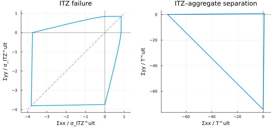

The ITZ envelope is symmetric about the diagonal   (dashed), as it must be for an isotropic material. Its edges are slightly curved: each corresponds to a family of points of the aggregate surface where the maximum moves as the load turns.

Sections of the ITZ envelope by deviatoric planes, at fixed values of the coordinate    along the hydrostatic axis, show the shape of the full surface in principal stress space. Each point is found by bisection on the deviatoric radius:

N3 = [1, 1, 1] / sqrt(3)       # hydrostatic axis
N1 = [-1, 1, 0] / sqrt(2)      # two deviatoric directions
N2 = [-1, -1, 2] / sqrt(6)
function section_radius(ξ, ψ; xmax = 8.0)
    S(x) = diagm(ξ * N3 + x * (cos(ψ) * N1 + sin(ψ) * N2))
    itz_peak(S(0.0)) ≥ 1 && return NaN      # beyond the hydrostatic limit
    lo, hi = 0.0, xmax
    for _ in 1:30
        mid = (lo + hi) / 2
        itz_peak(S(mid)) < 1 ? (lo = mid) : (hi = mid)
    end
    return lo
end
ψd = range(0, 2π; length = 73)
p = plot(; aspect_ratio = :equal, xlabel = "along N₁", ylabel = "along N₂",
    legend = :outerright, title = "Deviatoric sections of the ITZ envelope")
for ξ in -2.0:0.5:1.0
    r = [section_radius(ξ, ψ) for ψ in ψd]
    plot!(p, r .* cos.(ψd), r .* sin.(ψd); lw = 2, label = "ξ = $ξ")
end
p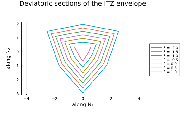

The sections shrink to a point as the hydrostatic tension grows, and widen under hydrostatic compression: a Rankine criterion in the ITZ makes concrete sensitive to the mean stress, with no friction law assumed anywhere. The surface they describe, in interactive form:

include(joinpath(pkgdir(MeanFieldHomogenization), "scripts", "common", "docviz.jl"))
direction(u, v) = cos(u) * N3 + sin(u) * (cos(v) * N1 + sin(v) * N2)
radius(u, v) = itz_limit(diagm(direction(u, v)))   # u: angle from the hydrostatic axis
ξcut = -5.0
ξapex = radius(0.0, 0.0)                            # hydrostatic tension
## Angle at which the meridian v crosses the deviatoric plane ξ = ξcut. The
## limit is infinite near hydrostatic compression, where the product is -Inf.
function u_cut(v)
    lo, hi = π / 2, π
    for _ in 1:40
        mid = (lo + hi) / 2
        radius(mid, v) * cos(mid) > ξcut ? (lo = mid) : (hi = mid)
    end
    return lo
end
## The meridian v, from the apex to the cut.
meridian(v; n = 41) = (uc = u_cut(v);
    [radius(t * uc, v) * direction(t * uc, v) for t in range(0, 1; length = n)])
vs = range(0, 2π; length = 73)
P = reduce(hcat, meridian.(vs))
surface = surface_trace(getindex.(P, 1), getindex.(P, 2), getindex.(P, 3);
    color = "#4a90d9", opacity = 0.85)
rim = line_trace(P[end, :]; color = FIG_VECTOR, width = 5)
axis = line_trace([(ξcut - 1) * N3, (ξapex + 1) * N3]; color = FIG_GUIDE, width = 3)

The six curved faces of the envelope (Königsberger et al., 2014; Fig. 4(b)) appear around the hydrostatic axis (gray line). The surface does not close under hydrostatic compression, so it is cut by the deviatoric plane   : each meridian is followed from the apex up to the angle at which it crosses that plane, found by bisection, and the rim of the surface is the section of the envelope by the plane. Along each direction the limit itself is exact, being positively homogeneous of degree one in .

Three families of planes cut it. The deviatoric planes   give back the sections of the previous figure. The planes   contain the hydrostatic point , inside the envelope as long as it lies below the apex, so that the section is found by bisection along the rays issued from it;   gives back the biaxial envelope drawn above (Königsberger et al., 2014; Fig. 7). Under lateral compression these sections reach beyond the cut of the surface, and that part of them is drawn in the panel only. The meridian planes contain the hydrostatic axis and the deviatoric direction    , where    and     are the in-plane axes of the previous figure; their sections are two meridians of the surface itself, and   is the plane   of axisymmetric triaxial tests.

ψc = range(0, 2π; length = 73)
points(cols) = reduce(hcat, cols)
dirN(ψ) = cos(ψ) * N1 + sin(ψ) * N2

## Deviatoric planes ξ = const.
ξs = filter(<(ξapex), -5.0:0.5:2.0)
rdev = [[section_radius(ξ, ψ; xmax = 20.0) for ψ in ψc] for ξ in ξs]
hdev = 1.15 * maximum(maximum(r) for r in rdev)
deviatoric = CutFamily(
    "Deviatoric plane", "ξ", string.(ξs),
    [plane_patch(ξ * N3, N1, N2, hdev, hdev) for ξ in ξs],
    [points(ξ * N3 + ri * dirN(ψ) for (ri, ψ) in zip(r, ψc)) for (ξ, r) in zip(ξs, rdev)],
    [points([ri * cos(ψ), ri * sin(ψ)] for (ri, ψ) in zip(r, ψc)) for r in rdev],
    ("along N₁", "along N₂"); active = findfirst(==(0.0), ξs),
)

## Planes Σ₃ = s, by bisection along the rays issued from (s, s, s).
function biaxial_point(s, ψ; xmax = 20.0)
    S(x) = [s + x * cos(ψ), s + x * sin(ψ), s]
    lo, hi = 0.0, xmax
    for _ in 1:40
        mid = (lo + hi) / 2
        itz_peak(diagm(S(mid))) < 1 ? (lo = mid) : (hi = mid)
    end
    return S(lo)
end
sbi = [s for s in -2.0:0.25:1.0 if sqrt(3) * s < ξapex]
cbi = [points(biaxial_point(s, ψ) for ψ in ψc) for s in sbi]
## On the surface, the part of a section beyond the cut is left out.
onsurface(C) = ifelse.(sum(C; dims = 1) ./ sqrt(3) .≥ ξcut, C, NaN)
lo, hi = extrema(vcat(getindex.(P, 1), getindex.(P, 2)))
biaxial = CutFamily(
    "Plane Σ₃ = s", "s", string.(sbi),
    [plane_patch([(lo + hi) / 2, (lo + hi) / 2, s], [1, 0, 0], [0, 1, 0], 0.55 * (hi - lo), 0.55 * (hi - lo)) for s in sbi],
    onsurface.(cbi), [C[1:2, :] for C in cbi],
    ("Σ₁ / σ_ITZ^ult", "Σ₂ / σ_ITZ^ult"); active = findfirst(==(0.0), sbi),
)

## Meridian planes: two meridians of the surface, joined at the apex.
ψm = 0:15:165
cme = [points(vcat(reverse(meridian(deg2rad(ψ) + π)), meridian(deg2rad(ψ)))) for ψ in ψm]
hme = 1.15 * maximum(maximum(abs, dirN(deg2rad(ψ))' * C) for (ψ, C) in zip(ψm, cme))
meridional = CutFamily(
    "Meridian plane", "ψ", ["$(ψ)°" for ψ in ψm],
    [plane_patch((ξcut + ξapex) / 2 * N3, N3, dirN(deg2rad(ψ)), 0.55 * (ξapex - ξcut), hme) for ψ in ψm],
    cme, [vcat(dirN(deg2rad(ψ))' * C, N3' * C) for (ψ, C) in zip(ψm, cme)],
    ("along cos ψ N₁ + sin ψ N₂", "ξ = √3 Σm"); active = findfirst(==(90), ψm),
)

section_figure([surface, rim, axis], [deviatoric, biaxial, meridional];
    uid = "itz-envelope-3d", height = 640, camera = (1.6, -1.6, 1.0),
    xlabel = "Σ₁ / σ_ITZ^ult", ylabel = "Σ₂ / σ_ITZ^ult", zlabel = "Σ₃ / σ_ITZ^ult",
    title = "Elastic limit of concrete by ITZ failure, principal stress space, cut at ξ = −5")

The buttons above the surface choose a family of planes, or none, and the slider below moves the plane; on the right, the section is drawn in coordinates of its plane, which is where the two-dimensional envelopes above are read.

Where to go next

The combined criterion of Königsberger et al. (2014) takes the lower of the two limits; which mode governs then depends only on the ratio , and the two functions of this page give it for any load. The jump conditions used here are those of Periodic multilayer — the laminate cell, applied to a single interface, and the pointwise fields of the coated sphere that converge to them are described in Layered sphere — pointwise fields. The next application, A lamellar porous material: swelling clays and C-S-H, moves to the geomaterials, whose grains interact through interfaces that slide.