Strength of a frictional matrix with a non-associated flow rule

The whole page as one script

Every block of this page, in order, is scripts/material_laws/18_frictional_strength.jl. From a clone of the repository, julia --project=docs -e 'using Pkg; Pkg.instantiate()' once, then julia scripts/material_laws/18_frictional_strength.jl, runs it end to end.

Soils, rocks, mortars and concretes have a strength that depends on the mean stress, and their plastic flow is usually less dilatant than the normality rule would make it. This page computes the macroscopic strength of a composite whose matrix obeys such a law, a Drucker–Prager criterion with a non-associated flow rule, around pores or rigid inclusions. The method is that of Maghous et al. (2009), which extends to non-associated plasticity the approach of Barthélémy and Dormieux (2003) for a von Mises matrix (the strength of a porous plastic solid). The equation numbers below are those of the 2009 paper. The example below runs it.

The matrix

The matrix can carry the stresses whose mean part and deviatoric norm   satisfy

eq. (1): is the isotropic tensile strength and the friction coefficient. Its plastic strain rate follows the potential   , eq. (15), so that away from the apex   , eq. (16), with the volume strain rate and the norm of the deviatoric one. The dilatancy coefficient lies between 0 and ; the normality rule is  . When   the theorems of limit analysis no longer hold, and the macroscopic limit states have to be defined otherwise.

A viscous matrix that tends to the plastic one

The limit states are defined as limits of the states of a sequence of viscous matrices indexed by   (§3.2 of the paper). Writing    , the matrix of index has the stress

eq. (17), where is a convex, twice differentiable function, zero for  , decreasing, and infinite at   . Its mean stress is    and the norm of its deviator  . The prestress    , eq. (19), is the one that places every stress on the criterion:       . Since   only for   , the flow rule    is reached as  .

The same stress reads as a linear law with strain-rate dependent coefficients, eqs. (20)–(22):

with positive moduli, since   and  . One checks that     , the mean stress found above.

The package takes      for    (and zero beyond), with  , which has the required properties; the limit states do not depend on this choice.

The modified secant method

The moduli and the prestress vary through the matrix with the local strain rate. As in the secant methods, the matrix is given uniform values, taken at effective strain rates: the square roots of the second moments of and over the matrix, eq. (25),  ,  . The matrix is then a linear viscous material with a uniform prestress, and the composite a linear one, whose second moments follow from the derivatives of its effective potential with respect to the moduli of the matrix, at fixed prestress:

being the fraction of the heterogeneities. Both equations form a fixed point on , which the package solves by Newton's method.

The effective potential of the composite with a prestressed matrix is exact in the two cases of the paper, for any linear scheme:

• Pores. A uniform prestress in the matrix is a uniform eigenstrain   there. The same eigenstrain in the pores changes nothing, since they carry no stress: it is a uniform eigenstrain of the whole cell, which only shifts the strain rate. Hence         with    , and the macroscopic stress is   . Its derivatives are those of eq. (45) of the paper, which is recovered for the Mori–Tanaka scheme.

• Rigid inclusions. The strain rate vanishes in the inclusions, so that the average of over the cell is :       and    , eqs. (33)–(34).

The derivatives of come from automatic differentiation through the scheme, so that nothing specific to a scheme or to a shape is written.

The limit states

As  ,      and  : the matrix of the comparison composite becomes nearly incompressible about the dilatant volume change  . The macroscopic stresses of the regularized composites tend to the limit states, at first order in . For spherical heterogeneities and the Mori–Tanaka scheme the paper finds the limit in closed form:

• porous medium: the elliptic domain of eq. (50),

  which does not depend on the dilatancy , while the macroscopic flow rule does: it derives from the potential of eqs. (53) and (55), the same ellipse with replaced by  . The flow is associated only if  .

• rigid inclusions: a Drucker–Prager cone, eq. (40),   , reached by strain rates that follow the macroscopic flow rule  , eq. (39), with

  Every point of the cone has the same normal, so that a strain rate fixes the point only through its distance, of order , to the flow rule. A strain rate off the flow rule has no limit state.

The tests of the package recover these closed forms from the general fixed point, and the von Mises limit ( ,   with fixed, eq. (56)) from the rigid–plastic secant composite.

Numerical notes and scope

regularization	is taken relative to  :     is nonnegative, so must stay below  . A dilatancy   is the limit of small and is refused
convergence	first order in ; two values of and a Richardson extrapolation remove most of the error; below a relative of about rounding takes over
heterogeneities	pores are given moduli times the smallest modulus of the matrix, rigid inclusions times the largest, since grows as
no limit state	a strain rate without one (rigid inclusions off the flow rule) drives the fixed point to the edge    of the regularized matrix, and is refused
cost	about 40 µs per limit state for a two-phase Mori–Tanaka cell
scope	a matrix and one kind of heterogeneity, pores or rigid inclusions, any scheme and shape of the package; a single effective strain rate for the whole matrix, which, as the paper notes, underestimates the strength of a porous medium in compression near the porosity

Example: porous and reinforced frictional solids

This example computes the macroscopic limit states of composites with a Drucker–Prager matrix whose flow is less dilatant than the normality rule, by the method of Maghous, Dormieux and Barthélémy, and compares them with the closed forms of Maghous et al. (2009).

A porous frictional solid

A solid with a tensile strength   and a friction coefficient   holds 15 % of spherical pores. Three dilatancy coefficients are compared, from the normality rule   to a nearly isochoric flow:

using MeanFieldHomogenization, TensND, Plots

φ, h, T = 0.15, 1.0, 0.3
rve = RVE()
add_phase!(rve, :M, Ellipsoid(1.0), Dict(:C => TensISO{3}(3.0, 2.0)); fraction = :rest)
add_phase!(rve, :P, Ellipsoid(1.0), Dict(:C => TensISO{3}(3.0, 2.0)); fraction = φ)
composite(t; a = 1e-2) = FrictionalComposite(rve, DruckerPrager(; h, friction = T, dilatancy = t);
    heterogeneities = Pores(), regularization = a)

code	theory
DruckerPrager(; h, friction, dilatancy)	the criterion     and the flow potential
Pores()	the phases other than the matrix carry no stress
regularization	the parameter of the viscous matrix, relative to
limit_stress(composite, D)	the limit state reached under the macroscopic strain rate

Each direction of the strain rate, from compaction to expansion, gives a point of the boundary. Two regularizations and a Richardson extrapolation remove the first-order error in :

𝟏 = Mandel{Float64}(1, 1, 1, 0, 0, 0)
shear = Mandel{Float64}(1, -0.5, -0.5, 0, 0, 0)
mean_dev(σ) = (m = sum(σ[1:3]) / 3; (m, sqrt(sum(abs2, σ - m * 𝟏))))
limit(t, D) = 2 * limit_stress(composite(t; a = 5e-3), D).σ - limit_stress(composite(t; a = 1e-2), D).σ
rates = [sin(θ) * 𝟏 / 3 + cos(θ) * shear for θ in range(-1.4, 1.4; length = 25)]

# The closed-form domain, eq. (50): A Σm² + B Σm + C + D Σd² = 0.
A, B, C, Dd = 3φ / (2T^2) - 1, 2(1 - φ) * h, -(1 - φ)^2 * h^2, (1 + 2φ / 3) / T^2
Σm_line = range(-(B + sqrt(B^2 - 4A * C)) / (2A), (-B + sqrt(B^2 - 4A * C)) / (2A); length = 300)
p = plot(Σm_line, [sqrt(max(-(A * x^2 + B * x + C) / Dd, 0)) for x in Σm_line]; lw = 2, color = :black,
    label = "closed form, eq. (50)", xlabel = "Σ_m / h", ylabel = "Σ_d / h", legend = :topleft)
for (t, marker) in ((0.3, :circle), (0.15, :diamond), (0.05, :utriangle))
    pts = mean_dev.(limit.(t, rates))
    scatter!(p, first.(pts), last.(pts); marker, ms = 4, label = "t = $t")
end
p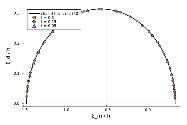

The three dilatancies give the same domain, as the paper predicts, and the points fall on the closed form. The domain is closed in compression: a porous solid ends up crushing its pores.

The flow rule depends on the dilatancy

The domain does not depend on , but the direction of the plastic flow at a given stress does. With the normality rule, the strain rate is normal to the domain; with  , it is normal to the plastic potential of eqs. (53) and (55), the same ellipse with replaced by :

θs = range(-1.2, 1.2; length = 9)
q = plot(Σm_line, [sqrt(max(-(A * x^2 + B * x + C) / Dd, 0)) for x in Σm_line]; lw = 2, color = :black,
    label = "", xlabel = "Σ_m / h", ylabel = "Σ_d / h", aspect_ratio = :equal)
for (t, color) in ((0.3, :steelblue), (0.05, :firebrick))
    for θ in θs
        D = sin(θ) * 𝟏 / 3 + cos(θ) * shear
        Σm, Σd = mean_dev(limit(t, D))
        Dv, Ddev = sum(D[1:3]), sqrt(sum(abs2, D - sum(D[1:3]) / 3 * 𝟏))
        n = 0.15 / hypot(Dv, Ddev)
        plot!(q, [Σm, Σm + n * Dv], [Σd, Σd + n * Ddev]; color, lw = 2, label = θ == first(θs) ? "flow direction, t = $t" : "")
    end
end
q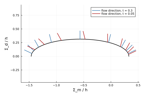

The arrows give the macroscopic strain rate at each limit state. For   they are normal to the domain. For a small dilatancy they lean toward the deviatoric axis: the porous solid flows with less volume change than the normality rule would give.

Rigid inclusions: a frictional cone

With rigid inclusions instead of pores, the limit states form a Drucker–Prager cone, eq. (40), whose friction coefficient grows with the fraction of inclusions and depends on the dilatancy. The strain rates that reach it follow the macroscopic flow rule  , eq. (39); the point on the cone depends on their distance to it, of the order of the regularization:

t_hom(φ, t) = t * sqrt((1 + 1.5φ) / (1 - 2φ * t^2 / 3))
T_hom(φ, t) = T * sqrt((1 + 1.5φ) * (1 - 2φ * t^2 / 3)) / (1 - 2φ * t * T / 3)
function friction(φ, t; offset = 0.4)
    cell = RVE()
    add_phase!(cell, :M, Ellipsoid(1.0), Dict(:C => TensISO{3}(3.0, 2.0)); fraction = :rest)
    add_phase!(cell, :R, Ellipsoid(1.0), Dict(:C => TensISO{3}(3.0, 2.0)); fraction = φ)
    D_on = t_hom(φ, t) * sqrt(1.5) * 𝟏 / 3 + shear
    T_of(a) = begin
        fc = FrictionalComposite(cell, DruckerPrager(; h, friction = T, dilatancy = t); heterogeneities = RigidInclusions(), regularization = a)
        Σm, Σd = mean_dev(limit_stress(fc, D_on - offset * a * t * sqrt(sum(abs2, D_on)) * 𝟏 / 3).σ)
        Σd / (h - Σm)
    end
    return 2T_of(5e-3) - T_of(1e-2)
end
fractions = range(0.05, 0.5; length = 10)
r = plot(; xlabel = "fraction of rigid inclusions", ylabel = "macroscopic friction T^hom", legend = :topleft)
for (t, color) in ((0.3, :steelblue), (0.05, :firebrick))
    plot!(r, fractions, T_hom.(fractions, t); color, lw = 2, label = "closed form, t = $t")
    scatter!(r, fractions, friction.(fractions, t); color, ms = 4, label = "computed, t = $t")
end
r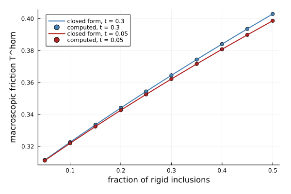

The inclusions raise the friction coefficient, more with the normality rule than with a nearly isochoric flow, and the computed values meet the closed form of eq. (40).

Going further

• Any scheme of the package replaces Mori–Tanaka (scheme = SelfConsistent()), and any shape of heterogeneity, with no closed form to compare with.

• The rigid–plastic secant composite is the von Mises limit of this one,   and   with fixed.

---

This page was generated using Literate.jl.