Crack opening displacement and compliance

Before this page

The Eshelby inclusion problem §2, where the tensor , which degenerates in a controlled way as the inclusion flattens, is introduced, and Concentration and contribution tensors §3 for the compliance contribution of a crack and its density.

A crack has no volume, so it cannot be described by a volume fraction and a stiffness. It is described instead by how much it opens under a given remote stress. That is the crack opening displacement tensor , and everything else on this page follows from it.

Read left to right: the COD tensor (order 2) gives the compliance contribution (order 4), which gives the dilute correction to the effective compliance; independently, gives the stress and displacement intensity factors , at the crack front.

MeanFieldHomogenization computes first — the intensity factors need it, and rebuilding from it avoids inverting a rank-deficient order-4 tensor. Its normalization is not unique in the literature, hence the Conventions section below.

1. Geometry

Elliptic and ribbon cracks

A crack is a plane region of unit normal , and two shapes of it are considered here: the ellipse and the ribbon , a strip of constant width extending without bound in one direction. Following Barthélémy (2026), both are described by one singular order-2 tensor , of rank 2 for the ellipse and 1 for the ribbon, whose kernel contains :

where   denotes the Moore–Penrose pseudo-inverse, the inverse itself being undefined for a singular tensor. Only   enters this definition, so that may be taken symmetric without loss of generality. With an orthonormal frame, the ellipse then corresponds to

and the second condition reads     : and are directed along the major and minor axes, and are the corresponding semi-axes, and the in-plane aspect ratio is   .

crack_figure(EllipticCrack(3.0, 1.5); uid = "th-cod-elliptic",
    title = "Elliptic crack ℰ, a = 3, b = 1.5 (η = 0.5)")

The ribbon is not the ellipse with  , which would be the segment of length carried by , but its limit as grows without bound while is held fixed. This limit is taken on the pseudo-inverse, the only part of the definition that remains finite, and it leaves

is thus invariant by translation along , of width , and its in-plane aspect ratio vanishes. Since the limit retains alone, the tensor no longer says how and are placed in the plane orthogonal to : one of them must be given in addition, which is why RibbonCrack stores the whole frame along with , and why a ribbon is better handled as the end of a family of ellipses than as a shape of its own.

crack_figure(RibbonCrack(1.5); uid = "th-cod-ribbon",
    title = "Ribbon crack ℛ, b = 1.5, unbounded along <u><i>ℓ</i></u>")

Both shapes are available as EllipticCrack(a, b), with PennyCrack(a) for the circle  , and RibbonCrack(b), oriented by Euler angles or by a given frame.

The crack as a degenerate ellipsoid

The compliance of a crack and its opening under load are obtained from the Eshelby problem of an ellipsoid (Conventions), the crack being regarded as an ellipsoid of vanishing thickness (Laws, 1977; Kachanov, 1992; Barthélémy, 2009). In the notation of Barthélémy et al. (2023) and Barthélémy et al. (2021), the ellipse is the limit of the ellipsoid

whose third semi-axis , along , is sent to zero, so that        is the rank-2 tensor of above. The slider of the figure lets decrease from 0.4 to 0.02:

flattening_figure(EllipticCrack(3.0, 1.5); uid = "th-cod-flat-ellipsoid",
    title = "Ellipsoid of semi-axes a, ηa, ωa around ℰ, a = 3, η = 0.5")

The ribbon requires both limits. Letting    first turns the ellipsoid into an elliptic cylinder of axis whose cross section has the half-axes along and along ; flattening that cross section then yields (Barthélémy et al., 2021). As is no longer finite, the flatness is measured on the cross section,

flattening_figure(RibbonCrack(1.5); uid = "th-cod-flat-cylinder",
    title = "Elliptic cylinder of half-axes b, ρb around ℛ, b = 1.5")

For the ellipse the same ratio reads   , and it is by that the limits defining the compliance of either crack are normalized in §3. On the code side, Ellipsoid(a, b, 0) and Ellipsoid(Inf, b, 0) return an EllipticCrack and a RibbonCrack respectively (degenerate limits).

2. The COD tensor

Under a remote stress , the two crack faces separate by the displacement jump . By linearity and the superposition principle, that jump depends on the loading only through the resolved traction   on the crack plane. Its average over the crack surface defines :

The normalization is by the in-plane half-width — the minor semi-axis of the ellipse, the half-width of the ribbon. This makes size-independent: it depends on the crack shape (through ) and on its orientation, never on how big it is. This is the convention of (Barthélémy, 2026), following Kachanov (1992), Kachanov (1993), and it is the one MeanFieldHomogenization implements (cod_tensor, alias B_tensor).

The shape coefficient

The opening profile is an ellipsoidal cap, so the average jump is a fixed fraction of the maximum jump at the crack center:

is worth introducing explicitly, because every numerical factor on this page comes from it. It is the one quantity that distinguishes the elliptic geometry from the ribbon one.

The 3-D → 2-D limit: a trap

A ribbon is the limiting shape of an ellipse as  , so one expects to be . It is not (Barthélémy, 2026):

The reason is exactly . The geometry does converge, and so does the pointwise opening profile; what changes is the relation between the average opening and the maximum one, because averaging over a shrinking ellipse is not the same operation as averaging across the width of a strip ( ). Since is defined from the average, it picks up the ratio  .

This matters in practice: the intensity factors of an elliptic crack are computed from the ribbon tensor of the tangent ribbon at each front point (see Intensity factors at the crack front below), so both objects appear in the same formula and must not be confused.

3. From to the compliance

The compliance contribution of a crack is defined from the ellipsoid, or the elliptic cylinder, of §1 as it flattens; is defined from the opening of the crack itself. This section proves that, with normalized by the half-width as in §2 and the flatness   of §1,

with      the second Hill tensor. The idea goes back to Kachanov (1992): the surface of a flat cavity becomes the two lips of the crack (Barthélémy, 2009; Barthélémy et al., 2021). It is written out here because both sides of the identity depend on two lengths, the one is normalized by and the one the flatness is measured on, which the sources choose differently (Conventions below).

Step 1: the strain a cavity adds is carried by its surface

A volume , of measure , of a linear elastic solid of stiffness   contains a cavity of volume , whose surface is free of traction, and is the unit normal to pointing out of the cavity. Its outer boundary carries the tractions   of a uniform stress , and its overall strain is the average of the boundary displacement:

The boundary of the solid   is and , the latter with the normal , so the divergence theorem gives

In the solid   , and the stress integrates to   over the solid: by the same theorem,   is the first moment of the tractions on the boundary, which are those of outside and vanish on the cavity. Hence

The strain added by the cavity is an integral over its surface alone; neither its shape nor its size has been used.

Step 2: an ellipsoidal cavity

Let be the ellipsoid of §1, alone in an infinite matrix, which is the dilute limit of (1). It is an inhomogeneity of zero stiffness, so by Eshelby's theorem the displacement of its surface is, up to a rigid motion, that of the uniform strain

A rigid motion adds nothing to the integral of (1), and     , so that

With (1), a cavity of volume fraction   adds   to the compliance: is the compliance contribution of a cavity (contribution tensors).

Step 3: the surface collapses onto the lips

Let the third semi-axis    tend to zero at fixed and (for the ribbon, the elliptic cylinder of half-axes and , per unit length along ). The volume vanishes like , and diverges like , but the surface integral (2) has a finite limit: the upper half of becomes the lip of facing , where   and  , and the lower half the lip facing , where    and  . With the area of and the definition of §2,

The last term is linear in . For any symmetric ,        , where the order-4 tensor has the components

Equating (2) and (3) for every ,

Step 4: the compliance contribution

Multiplying (4) by   ,

and is a number set by the shape alone:

	surface	volume
elliptic (3-D)
ribbon (2-D), per unit length

Both factors are independent of , which is the point of normalizing both and the flatness by : one definition covers the 2-D and the 3-D geometry, and inherits 's independence of size.

Step 5: the dilute correction, and back from to

cracks per unit volume (per unit area for ribbons) add, by step 2,   to the compliance, whose limit (4) is      :    for the ellipse and   for the ribbon, the crack densities of §6.

The map     loses nothing on a symmetric , which the COD tensor is: in a frame where  , the components of the image are   . is therefore read back from , and the bridge works both ways: compliance_from_cod and cod_from_compliance (src/Cracks/cod_H_bridge.jl), each the exact inverse of the other, apply the factor of the shape family of the crack.

Conventions: what and are normalized by

Steps 1 and 2 involve no convention. Step 3 uses two lengths: the one the mean opening is divided by in the definition of , and the one the flatness is measured on. MeanFieldHomogenization takes the half-width for both, as Barthélémy (2026) does for . Barthélémy et al. (2021) and Barthélémy et al. (2023) take the semi-major axis for an elliptic crack: their mean opening is and their flatness    . Steps 3 and 4 with in place of give

the factor holds in either convention, while the tensors of an elliptic crack differ by . The ribbon has no length , and the sources normalize it by as this package does. Echoes follows the elliptic normalization by and returns :

convention	elliptic	ribbon
MeanFieldHomogenization, of Barthélémy (2026):
Barthélémy et al. (2021), Barthélémy et al. (2023), Echoes: for the ellipse		as in MeanFieldHomogenization

They coincide for the penny crack  , which is why the discrepancy is invisible on the most common test case — and why a penny-only cross-check cannot detect a wrong -dependence.

Measured, not inferred from the papers — Echoes' crack_compliance against inverse_property_contribution on a flat triaxial ellipsoid ( ,  ,  ):

	1.0	0.7	0.5	0.3	0.1
	1.0000	0.7000	0.5000	0.3000	0.1000

On the MeanFieldHomogenization side the is -independent to machine precision (  for every ).

Check the normalization before comparing across sources

For an elliptic crack, the and of Barthélémy et al. (2021) and Barthélémy et al. (2023), and the that Echoes returns (it never forms ), are times those of this package and of Barthélémy (2026). Whether you compare a or an , check the normalization first.

Checking without going through

The closed forms of the next section give , and follows from it by the . Comparing to those closed forms would therefore verify nothing: it is the same formula read twice.

Read from right to left the boxed definition is a recipe: take a flat ellipsoid, compute , assemble     , invert, scale by the flatness  . That path never touches the crack machinery, so agreement with inverse_property_contribution is evidence rather than tautology:

using MeanFieldHomogenization, TensND, LinearAlgebra, Plots
gr()  # headless backend; GKSwstype is set to "100" in make.jl

E, ν = 210.0, 0.3
C₀ = TensISO{3}(E / (1 - 2ν), E / (1 + ν))   # (3k, 2μ)

## ρ-family of the definition, evaluated at finite flatness
function H_from_hill(a, b, ρ, C₀)
    Q = second_hill_tensor(Ellipsoid(a, b, ρ * b), C₀)   # ℚ = ℂ₀ − ℂ₀:ℙ:ℂ₀
    return ρ * inv(Q)
end

relerr(A, B) = norm(A - B) / norm(B)   # Frobenius norm, basis-independent

ρs = exp10.(range(-1, -3; length = 9))
plt = plot(; xscale = :log10, yscale = :log10, legend = :topleft,
           xlabel = "flatness ρ = c/b", ylabel = "relative error on ℍ")
for η in (1.0, 0.5, 0.3)
    crack = η == 1.0 ? PennyCrack(1.0) : EllipticCrack(1.0, η)
    H_ref = inverse_property_contribution(crack, C₀)
    plot!(plt, ρs, [relerr(H_from_hill(1.0, η, ρ, C₀), H_ref) for ρ in ρs];
          marker = :circle, label = "η = $η")
end
plot!(plt, ρs, ρs; linestyle = :dash, color = :black, label = "slope 1")
plt

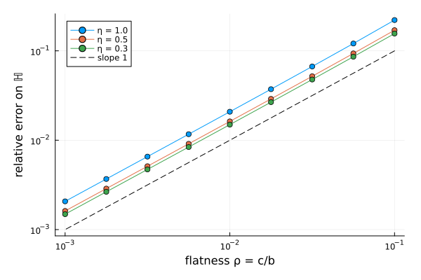
The three curves are straight lines of slope 1: the error decays like , which is the order of the Taylor term that resolves the limit (Barthélémy, 2009). That slope is the real content of the check — a single would not distinguish a true limit from a coincidence.

How flat the flattening route goes

The sweep stops at  . Both numerical back-ends hold far below it: at   the residues agree with the cubature to . None of this concerns cod_tensor, which resolves the limit analytically instead of flattening an ellipsoid.

Every route, in a triclinic matrix

In a matrix without any symmetry, comes from the reduced kernel of section 4 by three integrators, and from the flattening above with the Hill tensor by three integrators. The flattening error being , the combination    cancels its first-order term and leaves . Each side is compared with the other through compliance_from_cod and cod_from_compliance:

import DECUHR, Integrals   # loads the `:decuhr` back-end
using Printf

KM = [210.0 80 75 5 4 3; 80 195 90 -2 3 -1; 75 90 220 1 -2 2;
      5 -2 1 60 2.5 1.5; 4 3 -2 2.5 65 -1; 3 -1 2 1.5 -1 55]   # Kelvin–Mandel
C_tri = TensND.from_mandel(KM, TensND.CanonicalBasis{3, Float64}())
crack = EllipticCrack(1.0, 0.5)
tol = (; abstol = 1.0e-12, reltol = 1.0e-10)

B_ref = cod_tensor(crack, C_tri; method = :nestedquadgk, tol...)
H_ref = compliance_from_cod(B_ref, crack)
function H_flat(method, ρ)   # (c/b) ℚ⁻¹ of the flattened ellipsoid
    Q = second_hill_tensor(Ellipsoid(1.0, 0.5, 0.5ρ), C_tri; method, tol...)   # ℂ − ℂ:ℙ:ℂ
    return ρ * inv(Q)
end

for m in (:residues, :decuhr)
    @printf "B by %-12s against :nestedquadgk   %.0e\n" m relerr(cod_tensor(crack, C_tri; method = m, tol...), B_ref)
end
for (m, ρ) in ((:nestedquadgk, 1.0e-4), (:residues, 1.0e-4), (:decuhr, 1.0e-2))
    H = (10 * H_flat(m, ρ / 10) - H_flat(m, ρ)) / 9
    @printf "H flattened, %-12s ρ = %.0e: on H %.0e, on B %.0e\n" m ρ relerr(H, H_ref) relerr(cod_from_compliance(H, crack), B_ref)
end

B by residues     against :nestedquadgk   2e-15
B by decuhr       against :nestedquadgk   4e-15
H flattened, nestedquadgk ρ = 1e-04: on H 1e-09, on B 6e-10
H flattened, residues     ρ = 1e-04: on H 1e-09, on B 5e-10
H flattened, decuhr       ρ = 1e-02: on H 1e-05, on B 5e-06

The three integrations of agree to rounding. The extrapolated flattening meets them to about with the cubature and the residues, and to about with DECUHR, taken at   and only, where it stays fast.

The tutorial Two routes to a crack takes the limit otherwise: from the first-order term of in , the route of Barthélémy (2009), with no extrapolation, in random anisotropic matrices and for several aspect ratios, and exactly in SymPy for an isotropic one.

4. From the Green operator to

The closed forms of the next section are usually quoted. They are in fact derivable in closed form from the Fourier Green operator, and knowing where each factor comes from is what tells you which anisotropies admit a closed form at all. The script scripts/09_cod_symbolic_green.jl carries out the whole derivation symbolically, with the shipped closed forms as its oracles.

The reduced kernel

With     the acoustic (Christoffel) tensor, the two Fourier kernels of the traction integral equation on the crack plane are (Kunin, 1983; Kanaun and Levin, 2009):

and the object the crack problem actually needs is the reduced transform — the Fourier transform of the restriction of to the crack plane (Barthélémy, 2026):

Two properties do all the work. Contracting twice with collapses the order-4 algebra to a 3×3 one,

which is the form every back-end evaluates (Core/green_helpers.jl). And is homogeneous of degree , so the singly contracted kernel decays like while the doubly contracted one decays like : the integral above converges as written, and is homogeneous of degree .

Three reductions, then the integral

The integrand is a rational function of whose denominator is , a sextic whose roots are the Stroh eigenvalues. Three structural reductions precede any integration:

1. Equivariance. When is invariant under rotations about — isotropic, or transversely isotropic with its axis along — so is the whole construction, since is also the integrated direction. One in-plane direction determines all of them.

2. Homogeneity. Degree factors out a single  .

3. Parity. The – block of the integrand is odd in and integrates to zero.

Together, with   and   :

For an isotropic matrix the sextic degenerates to  , leaving the single pair of double poles   , and the three coefficients are just the plane-strain and antiplane moduli, derived step by step in The isotropic matrix, from the kernel to :

For a transversely isotropic matrix with the crack in the plane of isotropy, every component , carries an odd number of indices and therefore vanishes: the antiplane (SH) polarization decouples, and the sextic splits into a quadratic and a biquadratic — solvable by radicals,

The radical of the published TI closed form (Hoenig, 1978; Barthélémy et al., 2021) is therefore nothing but the sum of the two in-plane Stroh roots — it comes out of the factorization rather than being postulated.

From the reduced kernel to , for any anisotropy

The opening of an open crack under a uniform remote stress is an ellipsoidal cap, of maximum . Carried through the traction integral equation, that profile gives a uniform traction on the crack,    , with (Barthélémy, 2026)

Since   , the definition of reads   . The kernel being homogeneous of degree , depends on the shape only, through       , and

These hold whatever the anisotropy of the matrix. The closed forms of the next section are their evaluations when is known explicitly; otherwise the contour integral is computed numerically. For the ribbon,   leaves    and the contour integral reduces to   .

Fourier conventions, the reduced transform and the ellipsoidal profile

The Fourier transform of a function on and its inverse are taken as

Splitting    in the inverse transform and integrating over first shows that the reduced transform     is the  -dimensional Fourier transform of the restriction of to the plane . A shift of leaves it unchanged, so it ignores any component of its argument along ; a change of variable   shows that it raises the degree of homogeneity by one, which is how , of degree , gives a kernel of degree .

The ellipsoidal opening enters through the transform of the hemispherical cap on the unit disc,

an elliptical crack being mapped onto the unit disc by its semi-axis tensor. Inserted in the integral equation, this transform is what turns it into the uniform traction   above (Barthélémy, 2026).

The crack-plane integral: where the elliptic integrals enter

On the crack contour      of Barthélémy (2026),  ,      and       , so that

The of the degree-1 homogeneity has canceled the of the two in-plane dyads. being even in , the cross terms are odd and integrate to zero over , which is why is diagonal in the crack frame. Exactly three angular integrals survive. The integrands being even and -periodic,  , and the change of variable    turns into :

with the complete elliptic integrals and the two combinations of Barthélémy (2026),

The second forms follow from   , which gives     and    , with   and  . In terms of the Legendre parameter    of Elliptic integrals,    and   ; _elliptic_CS returns .

Hence

with the shape coefficient of the section above. The elliptic block is the same for the isotropic and the aligned-TI matrix — only change. That is why the two closed forms of the next section share one skeleton.

For the ribbon the contour integral is replaced by the single direction  , so   , and with  :

This is the exact identity behind the SIF ↔ DIF exchange relation at the end of this page: the operator that trades for is .

The isotropic matrix, from the kernel to

The steps above, carried out for      , end on the closed form of . Each line was checked by computer algebra.

1. The three tensors of the kernel. With    and   ,

and      with      .

2. The doubly contracted kernel. In the orthonormal frame ,        has the components

and   . All decay as , as announced.

3. The integral over . is odd in and integrates to zero. The three others need only

so that, with the factor of the reduced transform,

4. The contour integral. With the angular integrals of the previous section,

using   .

5. The inversion. is diagonal in the crack frame, and  :

the form of Barthélémy (2026). Replacing and by their expressions in and ,

gives the form of the next section.

6. The two limits. At the circle,    and  , so    and    . For the ribbon,  , where   and   : ``b\boldsymbol{\Lambda}^{\mathcal{R}} = a_2,\underline{\ell}\otimes\underline{\ell}

• a_1,\underline{m}\otimes\underline{m} + a_3,\underline{n}\otimes\underline{n}``,

and with  

What breaks in the general case

Nothing above survives a general anisotropy: the acoustic tensor no longer block-decouples, is an irreducible sextic in , and the crack plane has no rotational symmetry left, so one in-plane direction no longer determines the others. Both integrals become numerical — which is what the Residue and cubature back-ends do, the first summing residues over the six Stroh roots located numerically.

5. Closed forms of

Isotropic matrix

For      with Young's modulus and Poisson ratio , in the crack frame — derived step by step in The isotropic matrix, from the kernel to :

with   and   the complete elliptic integrals of the first and second kind (Abramowitz and Stegun, 1972), provided by ell_K and ell_E.

Near the circle

and , written with and , cancel as  ; they are evaluated by series there. And , a function of the ratio of the smaller semi-axis to the larger, has a kink at the circle, where the two swap roles: its derivative there is one-sided. Degenerate shapes gives both.

In terms of the combinations and of §4, which make both limits immediate (Barthélémy, 2026),

The three components are the three fracture modes: opens the crack (mode I), and shear it (modes II and III).

Penny crack  , where   :

Ribbon crack, with    and  :

Implementation: src/Cracks/cod_analytical.jl, selected by method = :auto when is a TensISO{4,3}.

Transversely isotropic matrix

When the matrix is transversely isotropic with its axis aligned with the crack normal , is still analytical. The closed forms are written in the engineering parameters of Hoenig (1978), defined on the compliance   in a frame whose third axis is :

With

the elliptic and ribbon COD tensors are (Hoenig, 1978; Kanaun and Levin, 2009; Barthélémy et al., 2021; Barthélémy, 2026)

They reduce to the isotropic forms above for    and   , where   and   . is the sum   of the two in-plane Stroh roots of §4. Implementation: src/Cracks/cod_analytical.jl, with the parameters read by TensND's ti_constants(…; form = :hoenig) from the compliance.

The stiffness components in the engineering parameters

With    , the five independent components that enter the reduced kernel of §4 are (Barthélémy, 2026)

the isotropic case giving    .

A transversely isotropic axis not aligned with the crack normal, and more generally a transformed transversely isotropic matrix, are treated in Barthélémy et al. (2023) for the compliance and the average opening, and in Barthélémy (2026) for the COD tensor and the intensity factors, by a linear transformation of the crack problem. Neither is implemented here.

Arbitrary anisotropy — numerical

No closed form exists in general. Following Barthélémy (2009), the limit   is resolved by extracting the first-order term of the Taylor expansion of in ; that term has an integral representation on the unit circle of the crack plane, evaluated by one of three algorithm traits:

• NestedQuadGK — nested adaptive Gauss–Kronrod quadratures, type-generic (src/Cracks/green_nestedquadgk.jl);

• DECUHR — adaptive cubature (Espelid and Genz, 1994), ForwardDiff-safe, once its weak dependency is loaded (src/Cracks/green_decuhr.jl);

• Residue — Cauchy-residue reduction to a 1-D quadrature, as in Masson (2008) adapted to the crack kernel, Float64 only (src/Cracks/green_residue.jl).

method = :auto picks NestedQuadGK, whatever the coefficient type and whatever else is loaded: it is the fastest and the most accurate of the three (see Hill polarization tensors). Residue degenerates when the reference is anisotropic in type and isotropic in value, a case the self-consistent and differential schemes reach at their first step, so it is available on explicit method = :residues only (src/Core/dispatch.jl).

6. Dilute correction to the effective compliance

inverse_property_contribution(crack, C₀) returns itself — the size-independent contribution, not the dilute correction. Cracks have no volume fraction, so the amount of cracking is measured by a Budiansky crack density (Budiansky and O'Connell, 1976; Kachanov, 1993), and reintroduced by delta_inverse_property:

	density	dilute correction
elliptic (3-D)	(number per unit volume × major × minor²)
ribbon (2-D)	(number per unit area × half-width²)

Implementation: src/Cracks/compliance.jl, dispatching on the crack shape.

7. Intensity factors at the crack front

At a point of the crack front, with in-plane outer normal and tangent   , the asymptotic expansions of the jump and the traction read (Irwin, 1957; Kassir and Sih, 1968; Willis, 1968):

is the displacement intensity factor (DIF) and the stress intensity factor (SIF), normalized so that the local energy release rate is simply    (Barnett and Asaro, 1972; Rice, 1989).

The central result of the anisotropic theory (Kanaun, 1981; Kunin, 1983; Kanaun and Levin, 2009) is that SIF and DIF are purely local and are exchanged by the COD tensor of the ribbon crack tangent to the real crack at the observation point:

This holds whatever the matrix anisotropy and whatever the remote loading — and it is why , with its factor, cannot be dispensed with even when studying elliptic cracks. With   (§4) it also reads    , and the energy release rate is a quadratic form in either factor (Barthélémy, 2026):

Elliptic crack

Parametrize the front by an angle :

with the in-plane semi-axis tensor and its pseudo-inverse. Then

where the dimensionless front factor is

The energy release rate follows as

Other parametrizations of the front

sif and dif take the front point through (keyword y₀, by default), the point itself being     . With the polar angle of , or the angle of the outer normal     , the front factor reads (Barthélémy, 2026)

from   and  . In terms of the maximum opening at the crack center,    and    .

Ribbon crack

Here    and  :

The SIF of an infinite ribbon crack is independent of the matrix stiffness — the of the DIF cancels against its inverse in the exchange relation — and the energy release rate is       .

Modes

Evaluation: sif and dif (src/Cracks/sif.jl).

8. Dispatch

(crack, C₀)	:auto selects	alternatives	ForwardDiff
EllipticCrack / RibbonCrack, TensISO	Analytical	—	✓
EllipticCrack / RibbonCrack, TensTI (aligned)	Analytical (MFH)	—	✓
EllipticCrack / RibbonCrack, AbstractTens{4,3}	NestedQuadGK	:residues, :decuhr, :nestedquadgk	✓

Entry points: cod_tensor / B_tensor for , inverse_property_contribution for , delta_inverse_property for , sif / dif for the front quantities. The transport counterpart — a scalar COD and a rank-1 resistivity contribution — is treated in Thermal cracks, with the same geometric factors and .

Where to go next

The transport counterpart is the next page, Thermal cracks, where a single scalar opening replaces and carries all the anisotropy of the matrix. The crack types and their densities are written as described in Cracks, and the tutorial Cracks and crack density places cracks in an RVE and follows the effective modulus as the density grows.