Ponte Castañeda–Willis

Before this page

Voigt and Reuss bounds, whose energy principles are refined here, Two-inclusion interaction tensors for the Green operator , its sign and the tensor through which one inclusion acts on another, and Mori–Tanaka, recovered below as a particular case.

Mori–Tanaka and Maxwell start from the solution of an inclusion problem and assemble it. The estimate of Ponte Castañeda and Willis (1995) starts elsewhere: from the energy of the composite, bounded by a variational principle, and from a statistical description of how the inclusions are distributed. The statistics enter through one ellipsoid per pair of phases, which describes how the centers of the inclusions of one phase are distributed around an inclusion of the other.

The derivation below is carried out for a matrix holding any number of inclusion phases, with these ellipsoids unrestricted. It builds the energy principle (§1), restricts it to a polarization uniform in each phase (§2), evaluates the statistical terms (§3) and solves the stationarity system (§4). The case of a single ellipsoid (§5), Mori–Tanaka (§6), the concentration tensors (§7) and the cracks (§8) follow, and §9 gathers the assumptions. The premises have nothing in common with those of the Maxwell scheme, with which the estimate nevertheless coincides in one case.

1. An energy principle with a comparison medium

The effective stiffness is defined by the effective energy, the minimum of the mean strain energy over the strain fields compatible with the affine displacement   on the boundary,

The principle of Hashin and Shtrikman (1962) compares the composite with a homogeneous medium of stiffness and energy     . Assume first softer than every phase, so that   is a convex function of the strain. Its Legendre transform,

gives, for every strain and every polarization field ,      . Taking the mean and the minimum over the admissible strains,

The remaining minimum is the problem of the homogeneous medium carrying the prescribed polarization . Its solution is the integral equation of the interaction page,

where is the convolution over the volume element. For a statistically homogeneous medium without long-range order, the kernel may be taken as the Green operator of the infinite medium, acting on the fluctuation of the polarization only, so that the strain averages to (Ponte Castañeda and Willis, 1995). With this solution, the stress    is in equilibrium and the strain fluctuation is compatible with zero mean, so their product averages to the product of their averages (Hill's lemma), and the minimum is            , and the effective energy is bounded below by the Hashin–Shtrikman functional

whatever . Its stationarity with respect to is the Lippmann–Schwinger equation with    : the exact polarization makes it an equality, and any other field gives a lower bound. When is stiffer than every phase,   is concave and the same steps, with the extremum reversed, make an upper bound. When is neither, the stationary value of over a restricted family of polarizations is an estimate, neither bound (Hashin and Shtrikman, 1963; Willis, 1977; Ponte Castañeda and Willis, 1995).

2. The matrix as comparison medium, a polarization per phase

The functional of §1 is exact only at the solution, which is unknown. An estimate follows from two choices: the comparison medium, and a family of trial polarizations small enough for the stationarity of to be solved over it.

The microstructure is a matrix of stiffness and volume fraction holding inclusion phases. All the inclusions of phase share the domain up to a translation (shape, orientation and stiffness ); inclusions of the same shape with another orientation form another phase. Their centers have the number density , so that   .

Taking the matrix as comparison medium makes   vanish in the matrix, where   is then infinite unless  : the polarization lives in the inclusions only. The family of polarizations searched is the simplest one, uniform in each phase and the same in every inclusion of that phase,

with the characteristic function of phase . The functional then becomes a quadratic function of the tensors ,

in which the microstructure enters only through the tensors . They depend on the moduli of the matrix and on how phase is seen from phase , that is on the two-point statistics.

3. Two-point statistics and the distribution ellipsoids

The remaining work is to express the tensors through the statistics of the inclusions. Writing each as the sum of the characteristic functions of its inclusions splits into two parts.

The self part. When the two points belong to the same inclusion, which requires  , the double integral over is times the self-interaction tensor , which is the Hill tensor for an ellipsoid. Summed over the inclusions of the phase, the self part is   .

The pair part. When the two points belong to two distinct inclusions, the part depends on where the inclusions of phase lie with respect to one of phase . Let be the number density of centers of phase at the separation from the center of an inclusion of phase . With the interaction tensor of such a pair, and the mean subtracted in , the pair part is

Three hypotheses make it computable (Ponte Castañeda and Willis, 1995):

1. the medium is statistically homogeneous, so that depends on the separation alone;

2. the statistics have ellipsoidal symmetry: depends on only through the norm attached to an ellipsoid centered on the origin, and vanishes inside it;

3. there is no long-range order: tends to fast enough as grows.

The symmetry of the statistics,     , requires  .

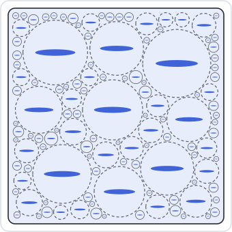
The figure shows a microstructure of this kind for one family of aligned flat inclusions and a spherical ellipsoid : each inclusion is centered in a sphere of half the size of , and these spheres do not overlap, so that no center comes closer to another than allows (§8).

Inside the density vanishes and the integrand reduces to   . Expanding the interaction tensor,   averages over and integrates over the integral of over , shifted by the difference between a point of and a point of . If every such difference lies in , the interior property of the Eshelby solution makes that integral equal to the Hill tensor of for every pair of points, and the contribution is          . The set of these differences,  , is exactly the set of separations at which an inclusion of phase and one of phase would overlap: the condition is that exclude overlaps.

Outside the bracket is constant on each ellipsoidal shell homothetic to . The Hill tensor of an ellipsoid does not depend on its size, so integrates to zero over the region between two homothetic ellipsoids that contain the point considered. Every shell therefore contributes nothing, and the decay of the third hypothesis makes the sum converge. Altogether,

For an inclusion that is not an ellipsoid, the same steps hold with replaced by its mean self-interaction tensor, the average of over the inclusion and over itself (Ponte Castañeda and Willis, 1995).

4. Stationarity and the estimate

With the tensors known, is an explicit quadratic function of the polarizations , and the estimate follows from its stationarity. Setting the derivative of with respect to each to zero, and dividing by , gives linear equations, written with    :

At the stationary point the quadratic terms of equal minus half its linear term, so that        , and the estimate is read off the mean polarization,    . Multiplying equation by writes the system with the block matrix of entries       , and

Since   and every is major-symmetric, is symmetric, and so is the estimate. When the matrix is the softest phase the estimate is a lower bound, and when it is the stiffest an upper bound, for the class of microstructures sharing these statistics; otherwise it is an estimate.

The equations can be read directly. Since    , equation says that   : each inclusion of phase has the polarization it would have if it were alone in the matrix, loaded at infinity by

The correction is the pair part of §3 read back: around the inclusion, phase is missing from , where its mean polarization   would otherwise be, and the beyond contributes nothing.

5. One distribution ellipsoid

The system of §4 has no closed-form solution in general, since each phase sees its own field . It has one when a single ellipsoid describes every pair,  : the field is then the same for every phase,    , and multiplying      by and summing leaves an equation for the mean polarization alone,      , and

the second form following from        . Expanded in the fractions, the estimate is the dilute one at first order, and the distribution enters at second order only, through    (Ponte Castañeda and Willis, 1995).

A coincidence with the Maxwell estimate

The second form is the Maxwell estimate of a domain shaped like . Nothing in either derivation announces it: one matches the far field of a cluster, the other makes an energy stationary over polarizations constrained by the statistics. It can be read after the fact, the remote strain applied to the Maxwell cluster being exactly the field    that each inclusion sees here, once the mean strain inside the cluster is taken as . It holds for one distribution ellipsoid only: a cluster has a single shape, and the Maxwell construction has no counterpart for distribution ellipsoids that depend on the pair of phases.

6. Mori–Tanaka as a choice of distribution

A single ellipsoid is not the only special case of the system of §4. Ponte Castañeda and Willis (1995) note that the Mori–Tanaka estimate follows formally from theirs, and trace its asymmetry with several inclusion shapes to an assumption on the distribution that violates the symmetry of the pair statistics. The pairwise system makes this explicit. Substituting  , the field     is the same for every phase, and the Mori–Tanaka solution satisfies the equations with that field equal to the mean strain of the matrix, since          . The choice is not symmetric in as soon as two phases differ in shape, so that loses its symmetry, and so does the estimate. It is symmetric, and the two estimates coincide, when every inclusion has the shape of the distribution.

7. Concentration tensors

The estimate is now complete, in general and in its two special cases. Unlike Mori–Tanaka, the derivation never used concentration tensors, but they follow from its stationarity condition. The mean of the strain that the integral equation of §1 produces in phase from the trial polarization is       , and the stationarity equation states that it equals   , the strain that the polarization of the phase stands for. The estimate of the mean strain of phase is therefore       , and writing   ,

The integral equation preserves the mean, so the matrix takes the rest,     , and      returns . With several distribution ellipsoids each phase has its own , given by the block system and without a closed form in general. With one ellipsoid they are all equal:

The field that loads the inclusions is the mean strain of the matrix when the bracket reduces to , as it does when every inclusion has the shape of the distribution: the Mori–Tanaka case again. The package implements the estimate with a single distribution ellipsoid, and concentration_tensors returns these tensors, the crack families of §8 entering as they do in the Maxwell estimate.

8. Cracks

Every phase so far has a volume. A crack family is the flat limit of a family of spheroids at a fixed density : its volume fraction vanishes while its polarization diverges, their product staying finite. Written on   , the system of §4 is regular in that limit,

and a crack family enters it with   replaced by   ,      , as in every other scheme of the chapter. Since a crack is softer than the matrix, a matrix holding cracks alone is its stiffest phase, and the estimate is an upper bound for its class within the admissible densities below. Its concentration tensor degenerates in the same way: the strain carried by the openings is     .

The condition that exclude overlaps limits the amounts that a given pair of shapes can describe. Take a single family of identical, aligned, centrally symmetric inclusions , for which    , and center on each of them the safety ellipsoid  . It contains the inclusion, since contains  . Two centers being separated by a vector outside , the safety ellipsoids do not overlap, and their fraction    cannot exceed one. The least restrictive choice is the smallest ellipsoid of the shape of that contains the inclusion, and   . For aligned spheroids of aspect ratio in a distribution of aspect ratio , the safety spheroid shares the axis of the inclusion, and

For penny-shaped cracks of radius the safety spheroid has the semi-axes  , and the density    is bounded by  : about 0.239 for a spherical distribution (Ponte Castañeda and Willis, 1995). Beyond that density no microstructure of the class exists, and the formula is no longer a rigorous bound. With a spherical distribution, the axial Young modulus of aligned cracks given by the estimate vanishes at  , beyond the admissible range (Ponte Castañeda and Willis, 1995). With a flat distribution of the same orientation as the cracks,  , the density limit recedes to infinity, and the estimate reduces to the non-interaction approximation, which Mori–Tanaka also gives for cracks (Ponte Castañeda and Willis, 1995).

9. Framework and limits

The assumptions met along the derivation delimit where the estimate can be used, and are worth checking before using it.

• A matrix–inclusion morphology: the matrix is the comparison medium and carries no polarization.

• A polarization uniform in each phase, the same in every inclusion of the phase. Once the statistics are fixed, this restriction of the variational principle is the only approximation.

• Two-point statistics only, homogeneous, without long-range order, and with ellipsoidal symmetry for each pair of phases,  .

• Impenetrable inclusions: each contains  , which caps the fractions and the crack densities (§8).

• A rigorous bound only when the matrix is the softest or the stiffest phase, and only for the class of microstructures sharing these statistics.

• Exact to first order in the fractions, the distribution acting at second order.

The package implements a single distribution ellipsoid, declared on the RVE (Distribution shape), and evaluates the second form of §5 with the kernel of the Maxwell scheme. It accepts there any inclusion that supplies a contribution tensor. For an inclusion that is heterogeneous, a layered sphere for instance, the polarization cannot be uniform in it, so the energy principle of §2 does not apply as such: the closed form evaluated is then that of the Maxwell scheme, whose far-field argument needs only the contribution tensor. The closed form has no iteration and accepts dual numbers and symbolic moduli, and the package evaluates the same kernel in conduction and in aging viscoelasticity.

Where to go next

Every scheme so far embeds the inclusions in the matrix. The next page, Self-consistent schemes, embeds each phase in the effective medium itself, which suits composites where no phase plays the role of a matrix.