
The differential scheme and path dependence
Before this page
The tutorial Bounds and classical schemes, where the differential scheme is placed among the other estimates, and the theory page The differential scheme, where the incorporation equation integrated below is derived.
The differential (or incremental) scheme builds a composite the way some real materials are actually made: by adding inclusions a little at a time, re-homogenizing after every increment. That construction history turns out to matter as soon as there is more than one inclusion phase.
The differential scheme
DifferentialScheme integrates the Norris differential equation (Norris, 1985) over a fictitious incorporation time
starting from
Trajectories for multi-phase RVEs
With a single inclusion phase, the trajectory is unambiguous: the fraction grows monotonically from 0 to its target value. With two or more inclusion phases, the order in which they are added along the way becomes a modeling choice, exposed through the trajectory keyword:
Proportional()(default) — every phase grows in lock-step, proportionally to its target fraction.Sequential(:A, :B)— phase:Ais added to completion first, then:Bis added into the resulting effective medium.Path(:A => τ -> ..., ...)— an arbitrary fraction-of-τschedule per phase, given as callables (CustomPathtakes tabulated values instead).
Seeing the path dependence
using MeanFieldHomogenization
using TensND
using LinearAlgebra
using Plots
gr()  # headless backend; GKSwstype is set to "100" in make.jl

C_m = iso_stiffness(30.0, 10.0)
C_stiff = iso_stiffness(60.0, 20.0)
C_soft = iso_stiffness(5.0, 2.0)

function build(f_total)
    r = RVE()
    add_phase!(r, :M, Ellipsoid(1.0), Dict(:C => C_m); fraction = :rest)
    add_phase!(r, :STIFF, Ellipsoid(1.0), Dict(:C => C_stiff); fraction = f_total / 2)
    add_phase!(r, :SOFT, Ellipsoid(1.0), Dict(:C => C_soft); fraction = f_total / 2)
    return r
end

trajectories = [
    (Proportional(), "Proportional", :black),
    (Sequential(:STIFF, :SOFT), "Sequential(STIFF, SOFT)", :blue),
    (Sequential(:SOFT, :STIFF), "Sequential(SOFT, STIFF)", :red),
]

fs = collect(range(0.005, 0.3; length = 25))
plt = plot(;
    xlabel = "total inclusion fraction f₁+f₂", ylabel = "k_eff",
    legend = :topleft, framestyle = :box, size = (760, 480),
)
for (traj, label, color) in trajectories
    ks = [k_mu(homogenize(build(f), DifferentialScheme(; trajectory = traj, nsteps = 100), :C))[1] for f in fs]
    plot!(plt, fs, ks; label = label, color = color, lw = 2)
end
plt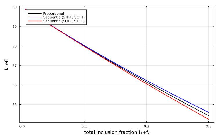
The three curves coincide in the dilute limit (small total fraction, where increments barely interact regardless of order) and fan out as the total fraction grows. Adding the stiff phase first leaves it embedded in a matrix that later softens further when the soft phase is added; adding the soft phase first has the opposite effect. Neither order is "more correct" in the abstract — the differential scheme encodes a construction history, and for a real composite the mixing or loading order is itself a physical modeling choice, not a numerical one.
Several trajectories, watched over the whole history takes this further: instead of reading off only the endpoint k_eff of a fraction sweep, it plots Path schedule — over the whole incorporation history.
Following the construction history
The scheme knows the effective property at every τ, not just at the end. differential_path returns the saved states, which is both cheaper and more informative than re-running homogenize for a series of target fractions:
rve = build(0.3)
τ, Cs = differential_path(rve, DifferentialScheme(; nsteps = 200), :C)

plt2 = plot(;
    xlabel = "incorporation time τ", ylabel = "modulus",
    legend = :topright, framestyle = :box, size = (760, 480),
)
plot!(plt2, τ, [k_mu(C)[1] for C in Cs]; label = "k_eff", lw = 2)
plot!(plt2, τ, [k_mu(C)[2] for C in Cs]; label = "μ_eff", lw = 2, color = :red)
plt2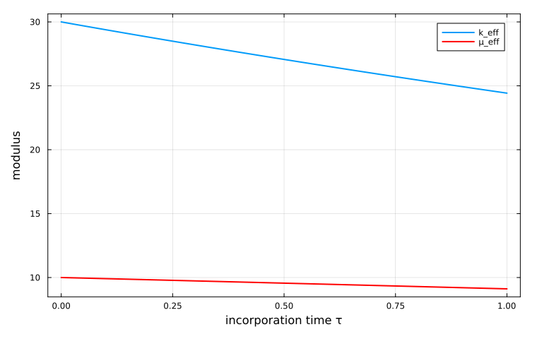
The curve is the actual construction history: reading it at τ = 0.5 gives the composite that has reached half of each target fraction, which is not the same as the composite built directly at those fractions unless the trajectory is proportional.
Several trajectories, watched over the whole history
The history above follows one trajectory and shows that the incorporation order matters, through the endpoint of a fraction sweep. Racing several trajectories to the same target fractions, and watching them the whole way through
A two-phase RVE with a strong contrast
To make the divergence between trajectories visible at a glance, the inclusions here are a genuinely stiff and a genuinely soft phase — a 5× contrast on each side of the matrix, rather than the milder pair used in the sections above:
using MeanFieldHomogenization
using TensND
using Plots
gr()  # headless backend; GKSwstype is set to "100" in make.jl

C_M = TensISO{3}(3 * 5.0, 2 * 2.0)          # matrix   : k = 5,  μ = 2
C_I1 = TensISO{3}(3 * 30.0, 2 * 12.0)       # phase I1 : stiff, 6× the matrix
C_I2 = TensISO{3}(3 * 0.5, 2 * 0.2)         # phase I2 : compliant, 0.1× the matrix
F1, F2 = 0.2, 0.2                            # target volume fractions

function build_rve()
    rve = RVE()
    add_phase!(rve, :M, Ellipsoid(1.0), Dict(:C => C_M); fraction = :rest)
    add_phase!(rve, :I1, Ellipsoid(1.0), Dict(:C => C_I1); fraction = F1)
    add_phase!(rve, :I2, Ellipsoid(1.0), Dict(:C => C_I2); fraction = F2)
    return rve
end
Four trajectories to the same target
Every trajectory below reaches f₁ = f₂ = 0.2 at τ = 1 — only the path taken to get there differs:
Proportional— both phases grow in lock-step.Sequential(:I1, :I2)— the stiff phase is incorporated to completion first, the soft phase second, into the resulting (already stiffened) medium.Sequential(:I2, :I1)— the reverse order.Path(:I1 => τ -> τ^2, :I2 => τ -> 2τ - τ^2)— a continuous schedule where:I1is backloaded (starts flat, catches up near :I2is frontloaded ([0, 1]with the required endpoints, but neither is proportional.
differential_path returns the full trajectory homogenize returns at τ = 1:
const NSTEPS = 200

function eval_path(traj)
    scheme = DifferentialScheme(; trajectory = traj, nsteps = NSTEPS, abstol = 1e-9, reltol = 1e-7)
    τ, Cs = differential_path(build_rve(), scheme, :C)
    kμ = k_mu.(Cs)
    return τ, first.(kμ), last.(kμ)
end

paths_to_run = (
    ("Proportional", Proportional(), :black),
    ("Sequential(I1 → I2)", Sequential(:I1, :I2), :blue),
    ("Sequential(I2 → I1)", Sequential(:I2, :I1), :red),
    ("Path (I1 backloaded, I2 frontloaded)", Path(:I1 => τ -> τ^2, :I2 => τ -> 2τ - τ^2), :green),
)

results = [(name, eval_path(traj)...) for (name, traj, _) in paths_to_run]
Watching the curves diverge
p_k = plot(; xlabel = "τ", ylabel = "k_eff(τ)", title = "Bulk modulus", legend = :right, framestyle = :box)
p_μ = plot(; xlabel = "τ", ylabel = "μ_eff(τ)", title = "Shear modulus", legend = false, framestyle = :box)
for ((name, _, color), (_, τ, k, μ)) in zip(paths_to_run, results)
    plot!(p_k, τ, k; label = name, color = color, lw = 2)
    plot!(p_μ, τ, μ; label = name, color = color, lw = 2)
end
plot(p_k, p_μ; layout = (1, 2), left_margin = 8Plots.mm, bottom_margin = 8Plots.mm, size = (1400, 600))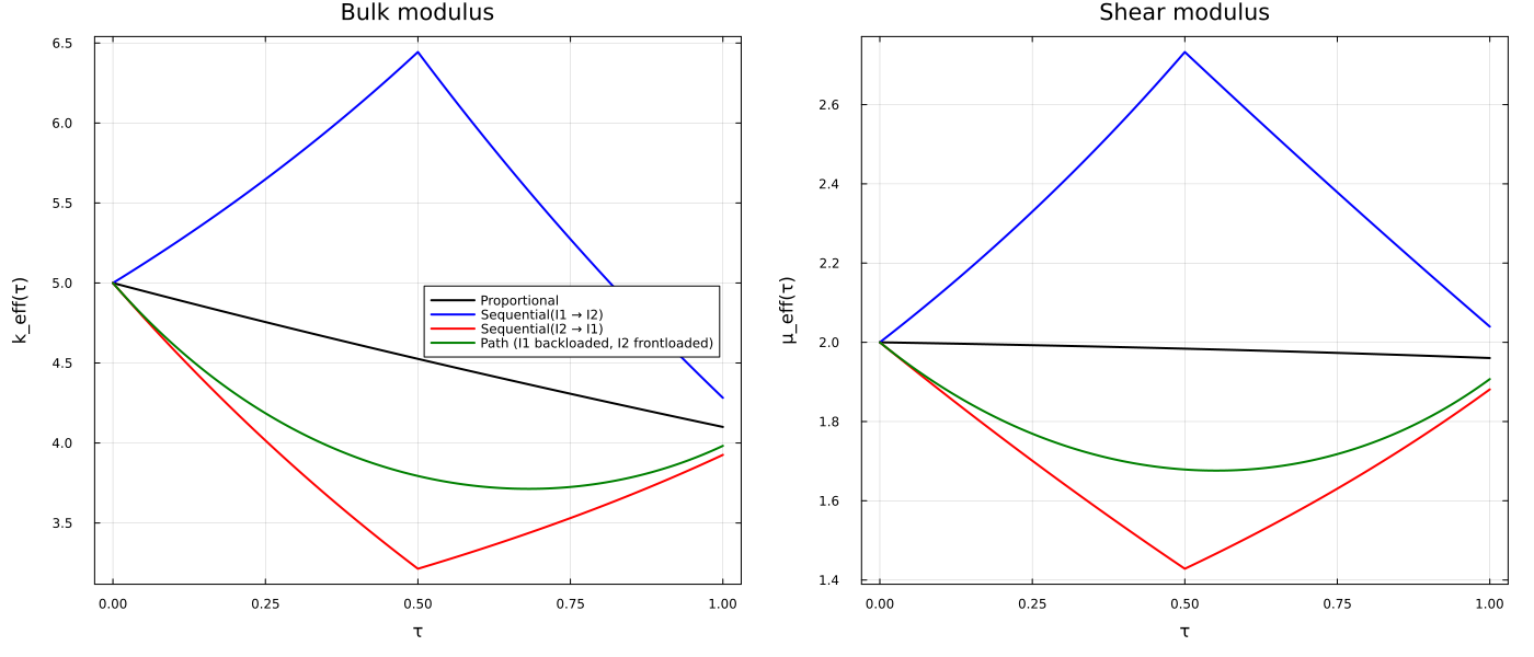
All four curves start together — in the dilute limit, the order in which two vanishingly small increments are added cannot matter — and pull apart as Sequential(I1, I2) ends up the stiffest of the four: the soft phase, added last, is diluted into an already-reinforced medium and does comparatively less damage than it would in a softer host. Sequential(I2, I1) is the mirror image and ends up the softest. The two Proportional and Path curves sit strictly between the two sequential extremes — expected, since every intermediate schedule interpolates between the two orderings in some sense — but they are not equal to each other, which is the point: the trajectory itself is a modeling choice, not just its start and end.
using Printf
for (name, _, k, μ) in results
    @printf "%-38s k_eff(1) = %.5f   μ_eff(1) = %.5f\n" name k[end] μ[end]
end
Proportional k_eff(1) = 4.10026 μ_eff(1) = 1.96032
Sequential(I1 → I2) k_eff(1) = 4.28232 μ_eff(1) = 2.03961
Sequential(I2 → I1) k_eff(1) = 3.92579 μ_eff(1) = 1.88116
Path (I1 backloaded, I2 frontloaded) k_eff(1) = 3.98228 μ_eff(1) = 1.90718A standalone, plain-Julia version of this comparison — same RVE, same four trajectories, writing a PNG instead of embedding it in the docs — lives in scripts/24_differential_loading_paths.jl.
Stiffness or compliance
The same ODE can be integrated on the compliance
rve = build(0.3)
tol = (abstol = 1e-12, reltol = 1e-10)
C_stiff = homogenize(rve, DifferentialScheme(; tol...), :C)
C_compl = homogenize(rve, DifferentialScheme(; formulation = :compliance, tol...), :C)
(k_mu(C_stiff), k_mu(C_compl))
((24.427350250070486, 9.114294430893029), (24.42735025004795, 9.114294430898399))The choice matters when the effective medium approaches a degenerate state: integrating C → 0 (porous or cracked media near percolation) is stiff in the stiffness variable and gentle in the compliance one.
Cracks
Cracks are the one case where the volume-replacement picture breaks down: their volume fraction vanishes (density and follow the trajectory like any other phase:
function cracked(ε)
    r = RVE()
    add_phase!(r, :M, Ellipsoid(1.0), Dict(:C => C_m); fraction = :rest)
    add_phase!(r, :CR, PennyCrack(1.0), Dict(:C => C_m); density = ε, symmetrize = :iso)
    return r
end

εs = collect(range(0.0, 0.6; length = 25))
ks = [k_mu(homogenize(cracked(ε), DifferentialScheme(), :C))[1] for ε in εs]

plot(εs, ks ./ k_mu(C_m)[1];
    xlabel = "crack density ε", ylabel = "k_eff / k₀",
    label = "differential", lw = 2, legend = :topright,
    framestyle = :box, size = (760, 480),
)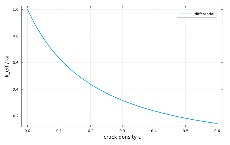
The differential scheme drives the stiffness towards zero without ever reaching it at finite density — no percolation threshold, unlike the self-consistent scheme, because each infinitesimal crack increment is introduced into an already-degraded medium.
Where to go next
Every scheme so far is an estimate. A stack of layers is the one cell solved exactly, with no Eshelby problem at all: Periodic multilayer: the exact laminate solution. The keywords of DifferentialScheme and of the trajectory types are collected in Homogenization schemes of the manual, and the crack density used in the last section is introduced in Cracks and crack density.