Dilute estimates

Before this page

Homogenization schemes, for the contribution tensors and , the identity that links them and the limits through which a crack family enters, and Voigt and Reuss bounds, the dual pair this page mirrors with an Eshelby problem in place of a uniform field.

The dilute estimates are the first to use the inclusion shapes. Each inclusion is placed alone in an infinite matrix, as if the others were absent, and loaded at infinity by the macroscopic field. Like the bounds, they come as a dual pair: the remote field is either the macroscopic strain or the macroscopic stress.

1. Dilute: the remote strain

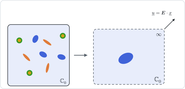
Taking   in the matrix gives   for every inclusion phase, and the average relation reduces to the sum of the contributions:

The assumption is consistent to first order only. With   the matrix keeps the macroscopic strain, and the strain average      differs from at order . The estimate is therefore exact as   and nothing more: it is linear in the fractions and in the crack densities, and for soft phases it loses positive definiteness at a finite amount. Spherical voids in an isotropic matrix, whose contribution has the spherical part     , bring the bulk modulus to zero at   .

2. DiluteDual: the remote stress

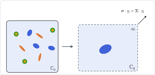
Prescribing the macroscopic stress at infinity instead adds the compliance contributions,

For cracks alone this is the non-interaction approximation of Kachanov and Sevostianov (2018): each crack opens under the remote stress as if it were alone, and the openings add up. It is the natural form for cracks, whose compliance contribution stays finite while the stiffness one is the limit of a diverging quantity. The package evaluates through     rather than through its definition, so that a void keeps the finite contribution it should.

3. The two estimates side by side

Since      , the two estimates agree to first order. Writing    ,

and their difference is      , which is positive semi-definite as long as itself is positive definite. The dilute estimate is thus always the softer of the two, whether the inclusions are stiffer or softer than the matrix. For spherical voids or rigid spheres in an isotropic matrix, the closed forms show that the Mori–Tanaka bulk modulus of the next page lies between the two.

4. Concentration tensors

Both estimates follow the construction of the overview, with the matrix as reference medium. Under Dilute the remote field is the macroscopic strain,  , and each inclusion keeps its dilute tensor,  . The matrix takes the rest of the average,

so that departs from at first order in the amounts, which is the inconsistency of §1 seen from the matrix. Under DiluteDual the remote field is the strain of the matrix under the macroscopic stress,     , hence    and    , the matrix again taking the rest. Its compliance contributions are then  : each inclusion of the dual estimate contributes to the compliance exactly as it does alone, which is the non-interaction approximation once more.

Where to go next

Both estimates ignore what surrounds an inclusion. The next page, Mori–Tanaka, keeps each inclusion in the matrix but loads it by the mean strain of the matrix, which restores the strain average at every fraction. The crack case is followed on a growing density in the tutorial Cracks and crack density.