
Porous materials: the self-consistent trap and every scheme
Before this page
The tutorial Bounds and classical schemes, which introduces the self-consistent scheme and the two bounds used below, and the theory page Self-consistent schemes, where the stiffness and compliance forms of the self-consistent iteration are stated.
Porosity is the simplest microstructure that breaks naive intuition: a pore is not "just a very soft inclusion" — it is an inclusion whose stiffness may vanish, and several schemes are not built to handle that limit gracefully. This page shows why, and introduces the scheme that was designed to.
Modeling a pore
A pore is modeled as an ordinary phase carrying a near-zero stiffness. Strictly zero stiffness makes the Reuss bound singular (it inverts
using MeanFieldHomogenization
using TensND
using LinearAlgebra
using Plots
gr()  # headless backend; GKSwstype is set to "100" in make.jl

C_solid = iso_stiffness(90.0, 30.0)
C_void = iso_stiffness(0.01, 0.005)   # soft, not exactly zero
Why the standard self-consistent scheme fails
SelfConsistent embeds every phase directly in the effective medium — including the pores. As porosity grows, the Picard iteration that solves the implicit self-consistent condition (see the previous tutorial) has to locate an effective stiffness soft enough to be consistent with soft, connected voids; near the percolation threshold the iteration becomes numerically unstable and can converge to an unphysical branch.
AsymmetricSelfConsistent fixes this by switching to the compliance-form iteration when the contrast calls for it — solving the dual condition on select_best = true keyword additionally keeps the best iterate seen during the loop, guarding against the Picard noise that can otherwise cross to the wrong branch near percolation. DiluteDual is the analogous dilute estimate for a soft phase: the natural dual counterpart of Dilute when it is the compliance, not the stiffness, that varies smoothly.
Schemes against the bounds
function bulk_at(f, scheme)
    r = RVE()
    add_phase!(r, :M, Ellipsoid(1.0), Dict(:C => C_solid); fraction = :rest)
    f > 0 && add_phase!(r, :V, Ellipsoid(1.0), Dict(:C => C_void); fraction = f)
    k, _ = k_mu(homogenize(r, scheme, :C))
    return k
end

fs = collect(range(0.0, 0.5; length = 61))
plt = plot(;
    xlabel = "porosity f", ylabel = "k_eff",
    legend = :topright, framestyle = :box, size = (760, 480),
)
plot!(plt, fs, [bulk_at(f, Voigt()) for f in fs]; label = "Voigt", color = :red, ls = :dash, lw = 2)
plot!(plt, fs, [bulk_at(f, Reuss()) for f in fs]; label = "Reuss", color = :gray, ls = :dash, lw = 2)
plot!(plt, fs, [bulk_at(f, MoriTanaka()) for f in fs]; label = "MoriTanaka", color = :green, lw = 2)
plot!(plt, fs, [bulk_at(f, DiluteDual()) for f in fs]; label = "DiluteDual", color = :blue, lw = 2)
plot!(
    plt, fs, [bulk_at(f, AsymmetricSelfConsistent(; abstol = 1.0e-10, maxiters = 200, select_best = true)) for f in fs];
    label = "AsymmetricSelfConsistent", color = :purple, lw = 2,
)
plot!(plt, fs, [bulk_at(f, DifferentialScheme(; nsteps = 100)) for f in fs]; label = "Differential", color = :orange, lw = 2)
plt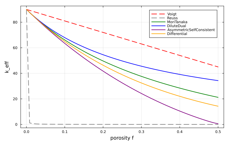
AsymmetricSelfConsistent and Differential sit comfortably between the bounds across the whole porosity range, while a naive SelfConsistent call on this same problem (try it — replace AsymmetricSelfConsistent above) becomes unreliable as f grows.
Every scheme on the whole porosity range
The bounds above stop at a porosity of one half. The canonical form of the benchmark, that of the Echoes book (Barthélémy, 2026), sweeps the entire range MeanFieldHomogenization implements, then flattens the pores.
The benchmark problem
using MeanFieldHomogenization
using TensND
using LinearAlgebra
using Plots
gr()  # headless backend; GKSwstype is set to "100" in make.jl

const k_s, μ_s = 72.0, 32.0        # solid moduli
const k_p, μ_p = 1.0e-6, 1.0e-6    # pore moduli (numerical regularization)

const C_s = iso_stiffness(k_s, μ_s)
const C_p = iso_stiffness(k_p, μ_p)
The microstructure the schemes are asked about, at a moderate porosity — drag to rotate. The second half of the page repeats everything with the pores flattened to
plotly_scene(rve_traces(; n = 70, semi_axes = (0.055, 0.055, 0.055),
        color = "#78909c", opacity = 0.95);
    uid = "pb-rve-spheres", height = 450,
title = "Spherical pores, isotropic distribution")plotly_scene(rve_traces(; n = 70, semi_axes = (0.075, 0.075, 0.015), seed = 7,
color = "#78909c", opacity = 0.95);
uid = "pb-rve-oblate", height = 450,
title = "Oblate pores, ω = 0.2, random orientations")Extracting effective moduli
The homogenized stiffness is expected to be isotropic here (spherical solid and pore geometry), so it can be read back directly with k_mu — as in the first tutorial. Some schemes can return a result with tiny numerical anisotropy (e.g. from an iterative solve that has not fully converged); dispatching to best_fit_iso first — the best isotropic projection of the tensor — keeps the extraction robust without changing the answer on already-isotropic input:
extract_kμ(C::TensND.TensISO{4, 3}) = k_mu(C)
extract_kμ(C::TensND.AbstractTens) = k_mu(best_fit_iso(C))
Every scheme at once
function build_rve(φ; ω_s = 1.0, ω_p = 1.0, sym_s = nothing, sym_p = nothing)
    r = RVE(; distribution_shape = Ellipsoid(1.0))
    add_phase!(r, :SOLID, Spheroid(ω_s), Dict(:C => C_s); fraction = :rest, symmetrize = sym_s)
    add_phase!(r, :PORE, Spheroid(ω_p), Dict(:C => C_p); fraction = φ, symmetrize = sym_p)
    return r
end

const SCHEMES = [
    (Voigt(), "Voigt", :red, :dash),
    (Reuss(), "Reuss", :blue, :dash),
    (MoriTanaka(), "Mori-Tanaka", :black, :solid),
    (SelfConsistent(; abstol = 1.0e-10, maxiters = 300, select_best = true), "Self-Consistent", :red, :solid),
    (AsymmetricSelfConsistent(; abstol = 1.0e-10, maxiters = 300, select_best = true), "Asym. SC", :purple, :solid),
    (DifferentialScheme(; nsteps = 100), "Differential", :gold, :solid),
    (Dilute(), "Dilute", :green, :dash),
    (DiluteDual(), "DiluteDual", :green, :dot),
    (Maxwell(), "Maxwell", :blue, :solid),
    (PonteCastanedaWillis(), "PCW", :green, :solid),
]

function sweep!(p_k, p_μ, scheme, label, color, ls, φs; build_kw = (;))
    ks, μs = Float64[], Float64[]
    for φ in φs
        try
            C = homogenize(build_rve(φ; build_kw...), scheme, :C)
            k, μ = extract_kμ(C)
            push!(ks, max(k, 0.0))
            push!(μs, max(μ, 0.0))
        catch
            push!(ks, NaN)
            push!(μs, NaN)
        end
    end
    plot!(p_k, φs, ks; lw = 2, color = color, linestyle = ls, label = label)
    plot!(p_μ, φs, μs; lw = 2, color = color, linestyle = ls)
end

φs = collect(range(0.0, 1.0; length = 51))

p_k = plot(; xlabel = "φ (porosity)", ylabel = "k_hom", xlims = (0, 1), ylims = (0, k_s + 5),
           legend = :topright, title = "Effective bulk modulus")
p_μ = plot(; xlabel = "φ (porosity)", ylabel = "μ_hom", xlims = (0, 1), ylims = (0, μ_s + 5),
           legend = false, title = "Effective shear modulus")

for (scheme, label, color, ls) in SCHEMES
    sweep!(p_k, p_μ, scheme, label, color, ls, φs)
end
plot(p_k, p_μ; layout = (1, 2), left_margin = 8Plots.mm, bottom_margin = 8Plots.mm, size = (1400, 600), plot_title = "Porous benchmark (spheres)")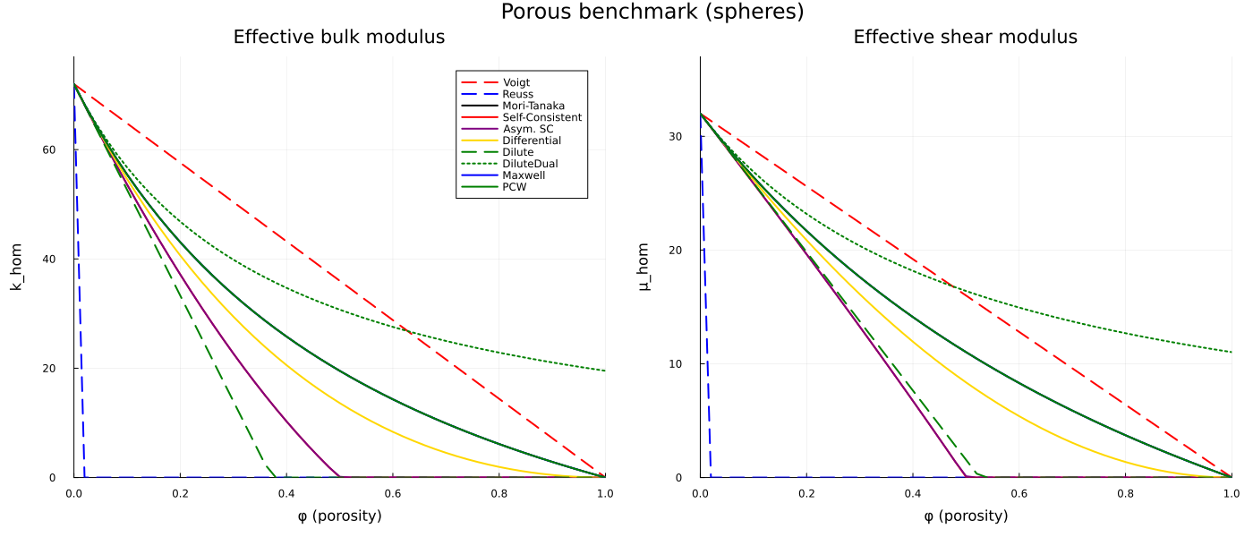
All schemes start at the solid's moduli and part ways in between:
| Scheme | Percolation | |
|---|---|---|
Voigt / Reuss | bracket the whole family | |
Mori-Tanaka, Maxwell, PCW | none — pores stay isolated inclusions | |
Self-Consistent, Asym. SC | ||
Differential | gradual |
select_best = true (see the previous tutorial) is what keeps the SC/ASC curves smooth through the crossover rather than jumping between branches under Picard noise.
Non-spherical pores
Real pore populations are rarely spherical. Replacing both phases with oblate spheroids (aspect ratio IsoSymmetrize() on each phase tells the homogenization kernel to average the concentration tensor over a uniform spatial distribution of orientations — so, even though each individual pore is anisotropic, the macroscopic effective tensor comes out isotropic:
const ω_oblate = 0.2

p_k2 = plot(; xlabel = "φ (porosity)", ylabel = "k_hom", xlims = (0, 1), ylims = (0, k_s + 5),
            legend = :topright, title = "Oblate pores (ω=$(ω_oblate)), iso-symmetrized")
p_μ2 = plot(; xlabel = "φ (porosity)", ylabel = "μ_hom", xlims = (0, 1), ylims = (0, μ_s + 5),
            legend = false, title = "Effective shear modulus")

for (scheme, label, color, ls) in SCHEMES
    sweep!(
        p_k2, p_μ2, scheme, label, color, ls, φs;
        build_kw = (; ω_s = ω_oblate, ω_p = ω_oblate, sym_s = IsoSymmetrize(), sym_p = IsoSymmetrize()),
    )
end
plot(p_k2, p_μ2; layout = (1, 2), left_margin = 8Plots.mm, bottom_margin = 8Plots.mm, size = (1400, 600), plot_title = "Porous benchmark (oblate + iso-symmetrize)")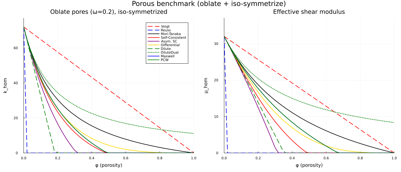
Numerical summary
for (scheme, label, _, _) in SCHEMES
    row = String[label]
    for φ in (0.0, 0.1, 0.3, 0.5, 0.7, 0.9)
        try
            k, μ = extract_kμ(homogenize(build_rve(φ), scheme, :C))
            push!(row, "$(round(k, digits=2))/$(round(μ, digits=2))")
        catch
            push!(row, "NaN/NaN")
        end
    end
    println(rpad(row[1], 16), join(rpad.(row[2:end], 14)))
end
Voigt 72.0/32.0 64.8/28.8 50.4/22.4 36.0/16.0 21.6/9.6 7.2/3.2
Reuss 72.0/32.0 0.0/0.0 0.0/0.0 0.0/0.0 0.0/0.0 0.0/0.0
Mori-Tanaka 72.0/32.0 55.44/26.42 33.46/17.63 19.53/11.02 9.9/5.88 2.86/1.77
Self-Consistent 72.0/32.0 53.61/25.87 22.69/13.26 0.08/0.06 0.0/0.0 0.0/0.0
Asym. SC 72.0/32.0 53.61/25.87 22.69/13.26 0.15/0.11 0.0/0.0 0.0/0.0
Differential 72.0/32.0 54.61/26.17 29.44/16.12 13.63/8.36 4.52/3.05 0.47/0.34
Dilute 72.0/32.0 52.65/25.91 13.95/13.73 -24.75/1.56 -63.45/-10.62 -102.15/-22.8
DiluteDual 72.0/32.0 56.75/26.88 39.86/20.37 30.72/16.4 24.99/13.72 21.06/11.8
Maxwell 72.0/32.0 55.44/26.42 33.46/17.63 19.53/11.02 9.9/5.88 2.86/1.77
PCW 72.0/32.0 55.44/26.42 33.46/17.63 19.53/11.02 9.9/5.88 2.86/1.77Every column reads k_hom/μ_hom at a fixed porosity — a compact way to compare all ten schemes at a glance. The try/catch guard around each evaluation matters in practice: a scheme that fails to converge at one particular porosity (rare, but possible near percolation) reports NaN there instead of aborting the whole sweep.
Where to go next
Every scheme above is evaluated in one shot or as a fixed point. The differential scheme and path dependence builds the composite incrementally instead, which makes the order of incorporation of the phases a modeling choice. The same porous medium carries a diffusivity as well as a stiffness, which Transport properties homogenizes with the same schemes at tensor order 2. The options of each scheme used in the sweep (tolerances, iteration caps, the select_best guard) are listed in Homogenization schemes of the manual, and the fixed-point iteration itself, with the Newton-type solvers that can replace it, is the subject of Nonlinear solvers for the self-consistent fixed point.