Layered sphere — bulk + shear recurrences and imperfect interfaces

Before this page

The Eshelby inclusion problem, whose uniformity result a composite pattern loses, and Concentration and contribution tensors, whose strain concentration tensor is what a pattern without a Hill tensor supplies instead, for the Homogenization schemes of the next chapter to consume.

LayeredSphere is an n-layer isotropic spherical composite inclusion in an infinite isotropic matrix, with per-layer concentration, global contribution tensors and layer / sphere / cumulative averages. The bulk and shear recurrences follow Hervé and Zaoui (1993) (generalizing the three-phase model of Christensen and Lo (1979)); imperfect interfaces follow (Hervé-Luanco, 2014) — PerfectInterface plus one primal/dual pair per physics:

Elasticity (primal / dual)	Conductivity (primal / dual)
SpringInterface(kn, kt)	KapitzaInterface(ρ)
MembraneInterface(κs, μs) surface elasticity (Dormieux et al., 2016)	SurfaceConductiveInterface(ks) (Barthélémy and Bignonnet, 2020)

1. Convention

Radii are stored in ascending order from the center,

with layer occupying   . Layer 1 is the core, layer is the outermost shell, and the composite sphere is embedded in an infinite matrix for  .

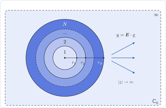
That is the whole problem the recurrences below solve: a concentric pattern in an unbounded reference medium , loaded by a remote uniform strain. Because the strain is not uniform inside such a pattern, it has no Hill tensor at all; what it does have is a volume-averaged concentration tensor, and that is what every scheme consumes.

The three-phase model of Christensen and Lo (1979) is one use of this solution rather than a variant of it — take   and let the reference medium be the unknown effective one, and the fixed point is their result. That is a property of the scheme, not of the pattern, so it lives with the schemes.

An interactive view of the layered geometry is in The inclusion zoo.

Moduli are TensISO{4,3} (elasticity) or TensISO{2,3} (conductivity). Interface conditions at each radius are specified in an NTuple{N, AbstractInterface} (default all PerfectInterface).

2. Bulk (spherical) recurrence — Hervé-Zaoui 1993

Under a purely hydrostatic remote strain, the displacement in layer is   , where and denote the bulk and shear moduli of the layer. To stay regular in the incompressibility limit  , the implementation propagates the field-valued state vector   directly, with the intra-layer transfer

where     and     with   . Every entry stays finite as   (hence also for  ), and the per-layer bulk concentration   degenerates smoothly (  for an incompressible core).

The entry-point at   is written in the "pressure amplitude" parameterization  , so that

3. Interface jump matrices

Each interface type provides a 2×2 (bulk) jump matrix such that   , on the state in elasticity and in conduction (§4). A jump is always the outer value minus the inner one,   . A spring interface is parametrized by its normal and tangential stiffnesses , , whose inverses  ,   are the compliances, a membrane by its surface bulk and shear moduli , , a Kapitza interface by its thermal resistance and a surface-conductive one by its surface conductance .

SpringInterface and KapitzaInterface encode a primal discontinuity (displacement / temperature jump), while MembraneInterface and SurfaceConductiveInterface encode a dual discontinuity (traction / flux jump). All limit to PerfectInterface when their compliance goes to zero.

The minus sign of the Kapitza matrix is that of the dictionary    of Conventions. The Kapitza law is the exact analog of the spring law   , namely   , and the state carries the physical outward normal flux , with    : hence    . Heat crossing the resistance outward leaves the inner side hotter than the outer one. With the interface would be a negative resistance, raising the conductance of the sphere it is meant to lower.

4. Conductivity recurrence (Y₁ harmonic)

Under a remote uniform temperature gradient, the temperature field has a Y₁ dependence,     with   . The state vector  ,     being the amplitude of the outward flux, propagates through a 2×2 transfer matrix    with  , being here the conductivity of the layer.

Interface jumps for conductivity are given above (Kapitza primal, SurfaceConductive dual, matching the structural pattern of their elastic analogs). The per-layer gradient concentration   reduces, in the single-layer case, to the classical   of Maxwell-type composites.

5. Type genericity & incompressibility

The recurrence consists of small-size matrix arithmetic over the element type; it is exercised with Float64, BigFloat, ForwardDiff.Dual, SymPyPythonCall.Sym, and Symbolics.Num. Symbolically,

using SymPyPythonCall; @syms κ₀ μ₀ κ₁ μ₁
s = LayeredSphere((Sym(1),), (TensISO{3}(3κ₁, 2μ₁),))
simplify(MeanFieldHomogenization.LayeredSpheres._bulk_concentration(s, κ₀, μ₀)[1])
# → (3κ₀ + 4μ₀) / (3κ₁ + 4μ₀)

and the derivative with respect to any modulus or radius is obtained by wrapping the computation in ForwardDiff.derivative / ForwardDiff.gradient.

6. Deviatoric (shear) recurrence — Y₂-harmonic 4×4 state vector

The bulk recurrence of §2 covers a hydrostatic remote strain only; the deviatoric part of the load calls for a second recurrence, on a four-component state vector.

Under a remote pure-deviatoric strain, the displacement field in an isotropic layer has the axisymmetric form   ,   , and the four linearly-independent Navier solutions at   are parametrized by the power-law exponents     with material- dependent ratios derived directly from the Navier characteristic equation (using  ):

Mode	Radial dependence
1		— uniform deviatoric strain
2
3
4

The corresponding traction amplitudes are obtained from Hooke's law      :

The state vector   combines displacement and physical traction amplitudes; this form is continuous across every perfect interface and rational in , so the recurrence is type-generic (supports Float64, BigFloat, ForwardDiff.Dual, SymPyPythonCall.Sym, Symbolics.Num) and remains regular in the incompressibility limit  .

Interface jumps at :

• Perfect: identity.

• Spring:    ,    , the traction being continuous.

• Membrane: a surface-elastic shell of moduli generates a jump in the tractions driven by the surface-stress divergence.

Seeding at uses the two regular modes (   and   ; the two singular amplitudes    are forced by regularity at the origin). Propagating both probes and solving a 2×2 linear system for the matrix-side far-field   yields the per-layer amplitudes.

The layer concentration is not the mode-1 amplitude alone. Mode 2 has an displacement profile, so it integrates to a non-zero deviatoric strain over a shell of finite thickness, whereas modes 3 and 4 average to zero pointwise:

Dropping the mode-2 term is invisible on degenerate configurations (vanishing core, core ≡ shell, single layer) and wrong by 1–50 % on a genuine multi-layer stack.

For   the recurrence reduces to the classical Eshelby single- sphere result; for   it reproduces the core-shell effective shear modulus of Christensen and Lo (1979) and passes the Eshelby consistency tests (  with core ≡ shell ↔ single-layer of radius , etc.).

7. Averages and interface jumps

7.1 Averages over the material

Three volume-average flavors are provided:

• layer_gradient_average(sphere, C₀, ε∞, k) — mean strain in layer (bulk + deviatoric parts).

• sphere_gradient_average(sphere, C₀, ε∞) — mean strain in the whole composite.

• cumulative_strain_average(sphere, C₀, ε∞, r) — mean strain inside the ball of radius .

All three cover the deviatoric part for any   via the shear recurrence above. They average the field over the material of the layers, which is what a local criterion needs. A spring interface adds strain that belongs to no layer, and the concentration tensor of the whole sphere has to count it.

7.2 The strain carried by a displacement jump

Over a ball of radius , the divergence theorem applied layer by layer gives

with the interface of radius , its outward normal and   . The left-hand side is the average over the material,  . The strain of the ball seen from outside is the first term on the right, read on the outer side of : it carries the opening of every interface. The two coincide only when no interface opens.

The strain average rule    requires each opening to be assigned to some phase. The concentration tensor of a composite sphere assigns to the sphere the openings of its inner interfaces, and of its outer one by default. This is also the convention of Echoes, of LayeredSpheroid and of the laminates.

On each harmonic the surface integral reduces to an amplitude. For the spherical part,    and      . For the deviatoric part, with  ,    and the remote strain of mode 1,       ,

since both angular integrals equal . Dividing by   and by   gives the weight of the part. Mode 1,  , then averages to 1 on its own ball, and modes 3 and 4 to zero on any shell, as §6 requires. The interface of radius therefore adds to the concentration of a ball of radius

per unit remote amplitude, on , on and in conduction. The jumps are those of §3 and §6:    in the spherical harmonic,    and    between amplitudes in the deviatoric one, and    . The traction and the flux are continuous across a primal interface, so the average stress and the average flux are unchanged. A jump is strain without stress, and it lowers the contribution tensor by  .

A single grain of bulk modulus bonded by a normal spring gives a check in closed form. Under a hydrostatic stress  , the grain strains by   in every direction and the interface opens by . The sphere seen from outside therefore strains by  , which is the response of a homogeneous grain of modulus

Its dilute concentration    is what the interface term restores. In conduction, the same reasoning gives    for a Kapitza resistance.

7.3 Which interfaces an average counts

Call	Inner interfaces	Outer interface	Echoes
gradient_gradient_concentration(sphere, C₀, C₀)	counted	counted	eE
gradient_gradient_concentration(sphere, C₀, C₀; external = false)	counted	not counted	sphere_eE(n-1, external=False)
gradient_gradient_concentration(sphere, C₀; layer = k)	—	—	layer_eE(k-1, external=False)
gradient_gradient_concentration(sphere, C₀; layer = k, external = true)	—	counted	layer_eE(k-1)
gradient_gradient_concentration(sphere, C₀; layer = k, internal = true)	counted	—	layer_eE(k-1, internal=True)
layer_gradient_average, sphere_gradient_average	—	—

external and internal keep the meaning they have in Echoes; only the default of the per-layer form differs, the material average. With external = true on every layer, the shells partition the sphere:   . The same keyword moves the surface stress of an outer membrane out of flux_gradient_concentration, so that     holds for either value. Conduction follows the same rules through gradient_gradient_concentration and flux_gradient_concentration. The schemes use the defaults.

These tensors reproduce Echoes to ten digits, with spring interfaces inside and outside the sphere, under Mori–Tanaka and the self-consistent scheme, and with Kapitza interfaces in conduction. In conduction they also match the spherical limit of the confocal spheroid, computed independently.

8. Pointwise fields

The recurrences above already carry everything needed to evaluate the field at a point, in any layer and in the matrix; only the reconstruction was missing. Write  ,   ,   .

Spherical part.    with   , hence     .

Deviatoric part. The general — non-axisymmetric —   solution is

which is the  ,    convention above through   ,  . Differentiating with    gives, with    ,

Every generator is transversely isotropic about — the configuration is rotation-invariant about the center — so the pointwise concentration tensor , defined by   , is a TensTI{4,T,6}: six Walpole coefficients and an axis, with no major symmetry.

Averaging over directions and over a shell returns exactly the above — mode 1 contributes , modes 3 and 4 contribute nothing pointwise, and mode 2 contributes  , whose shell average is the factor. shell_concentration exposes that identity from the same cached amplitudes, so the pointwise and averaged routes cannot drift apart.

The transport problem is the analog:     and        , a second-order transversely isotropic tensor.

Everything is validated pointwise against the C++ reference (Echoes' conc_eE, conc_eS, conc_sE, conc_sS) to , perfect, spring and Gurtin–Murdoch membrane interfaces alike.

See the worked example with figures: n-layer sphere: pointwise fields.

Where to go next

The next page, Layered spheroid, solves the same problem in conduction for confocal spheroidal layers, on which an imperfect interface couples the harmonic degrees that a sphere keeps apart. The per-layer concentration tensors of §7 are computed on a random multilayer in the tutorial n-layer sphere: volume-averaged concentration tensors, and the syntax of a layered inclusion is in Layered inclusions.