A first homogenization

Before this page

Getting started, where the package is installed and a first effective stiffness is read back, and the theory page Dilute estimates and Mori–Tanaka, where the estimates compared below are derived.

Every MeanFieldHomogenization computation starts from the same three ingredients: a representative volume element (RVE) describing the phases, their geometry, and a scheme that turns the RVE into a single effective property. This page builds the simplest possible RVE — a matrix with one spherical inclusion phase — and computes its effective stiffness two different ways.

Building an RVE

using MeanFieldHomogenization
using TensND
using LinearAlgebra
using Plots
gr()  # headless backend; GKSwstype is set to "100" in make.jl

rve = RVE()
add_phase!(rve, :M, Ellipsoid(1.0), Dict(:C => iso_stiffness(30.0, 10.0)); fraction = :rest)
add_phase!(rve, :I, Ellipsoid(1.0), Dict(:C => iso_stiffness(60.0, 20.0)); fraction = 0.2)
rve

RVE{Float64} with 2 phase(s)
  phase :M   f = 0.8  (rest)
  phase :I   f = 0.2
  closure : ComplementFraction(:warn)
  distribution_shape : none declared (Maxwell / PCW will ask for one)

RVE() creates an empty container; add_phase! then attaches a geometry (here Ellipsoid(1.0), a unit sphere), a property dictionary and an amount to each phase. fraction = 0.2 means 20 % of the RVE by volume; fraction = :rest means "whatever the others leave", here 80 %.

Note that nothing so far says which phase is a matrix — that is the scheme's to decide, and MoriTanaka() below takes the :rest phase because it is the only candidate. See Who is the matrix?.

A storage convention worth knowing

iso_stiffness(k, mu) builds the isotropic stiffness tensor from the physical bulk and shear moduli and . Internally TensND stores an isotropic 4th-order tensor as the raw pair — so TensISO{3}(a, b) interprets its two arguments as that pair directly, not as :

C1 = iso_stiffness(30.0, 10.0)      # from physical (k, μ) = (30, 10)
C2 = TensISO{3}(3 * 30.0, 2 * 10.0)  # same tensor, built from the raw pair
C1 == C2

true

Recover the physical moduli from either with k_mu:

k_mu(C1)

(30.0, 10.0)

To avoid this trap, every example in these tutorials builds isotropic stiffnesses with iso_stiffness(k, mu) and reads results back with k_mu.

The dilute estimate

The simplest scheme, Dilute, assumes each inclusion sits in an infinite matrix, ignoring every other inclusion around it. The effective stiffness is a sum of independent contributions:

where is the Hill polarization tensor of inclusion in the matrix (hill_tensor) and is its dilute strain-concentration tensor: the linear map from the macroscopic strain to the strain inside inclusion . This is exact only in the dilute limit   — at finite volume fraction, inclusions interact and the estimate drifts.

Mori–Tanaka: accounting for interaction

MoriTanaka corrects for this by loading each inclusion not with the macroscopic strain, but with the average strain in the matrix:

Both schemes are called the same way — only the scheme argument to homogenize changes:

k_dil, _ = k_mu(homogenize(rve, Dilute(), :C))
k_mt, _ = k_mu(homogenize(rve, MoriTanaka(), :C))
(k_dil, k_mt)

(33.54545454545455, 33.86138613861386)

Comparing the two across volume fraction

function build(f)
    r = RVE()
    add_phase!(r, :M, Ellipsoid(1.0), Dict(:C => iso_stiffness(30.0, 10.0)); fraction = :rest)
    add_phase!(r, :I, Ellipsoid(1.0), Dict(:C => iso_stiffness(60.0, 20.0)); fraction = f)
    return r
end

fs = exp10.(range(-4, log10(0.6); length = 30))
k_dil = [k_mu(homogenize(build(f), Dilute(), :C))[1] for f in fs]
k_mt = [k_mu(homogenize(build(f), MoriTanaka(), :C))[1] for f in fs]

plt = plot(;
    xlabel = "inclusion volume fraction f", ylabel = "k_eff",
    xscale = :log10, legend = :topleft, framestyle = :box, size = (760, 480),
)
plot!(plt, fs, k_dil; label = "Dilute", lw = 2)
plot!(plt, fs, k_mt; label = "MoriTanaka", lw = 2)
hline!(plt, [k_dil[1]]; label = "matrix", lw = 1, color = :gray, ls = :dash)
plt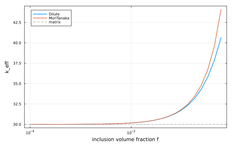

The two curves coincide as   — both schemes agree in the dilute limit, as they must — and diverge as grows: at finite volume fraction the inclusions interact, and Mori–Tanaka, which accounts for that, departs from the naive dilute sum.

Where to go next

The dilute and Mori–Tanaka estimates are two members of a larger family, which Bounds and classical schemes places on a single graph between the Voigt and Reuss bounds. The syntax of the RVE and of the scheme objects used above is collected, call by call, in Homogenization schemes of the manual.