Maxwell

Before this page

Mori–Tanaka, whose second form is compared with the estimate below, the sign of the Green operator fixed in the Conventions, and Concentration for the contribution tensors.

Mori–Tanaka describes what surrounds an inclusion by the mean strain of the matrix alone. The Maxwell scheme keeps the matrix as reference medium and adds a second shape: that of a domain which holds the inclusions and which, filled with the effective medium, must disturb the matrix far away as the inclusions do. The argument rests on nothing but the far field of an inhomogeneity, which this page derives from the Green operator of the matrix (§1) before building the estimate on it (§2) and reading the concentration tensors off the construction (§3).

The notation is the intrinsic one of Barthélémy et al. (2019), who transpose the scheme to aging viscoelasticity. It is written here in elasticity, with the conventions of this documentation: is a compliance, and the Green operator of the matrix maps a polarization onto minus the strain it induces.

1. The field of one inhomogeneity, seen from afar

An inhomogeneity occupies a bounded domain of any shape, with a stiffness that need not be uniform, and is embedded in the infinite matrix loaded at infinity by the strain . Its polarization     vanishes outside , and the Lippmann–Schwinger equation gives the strain everywhere:

At a point far from compared with its size, the kernel varies little across the domain, and   may be replaced by , the origin being taken inside . The leading term of the disturbance is then

because the mean polarization of the inhomogeneity is, by definition of its stiffness contribution,      . Since the matrix carries      and      , the same term reads, in stress,

At leading order, the far field thus depends on the inhomogeneity through a single product,   or equivalently  : its shape, its moduli and its inner structure enter nowhere else (Sevostianov and Kachanov, 2011). For an ellipsoid of uniform stiffness and Hill tensor ,    .

2. A cluster and its effective twin

Since the far field retains a single product per inhomogeneity, a set of inhomogeneities and a homogeneous domain can disturb the matrix in the same way. The scheme requires precisely that.

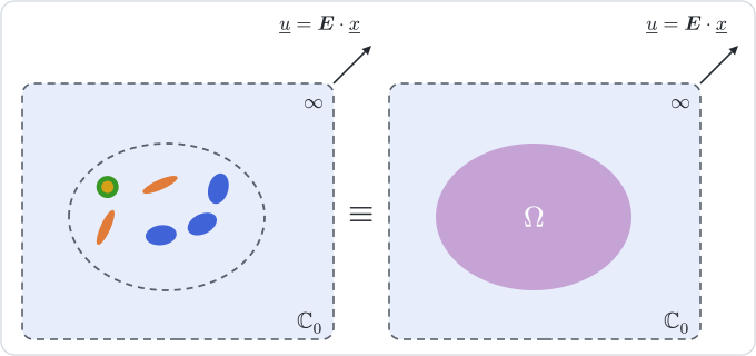
Cut out of the composite an ellipsoidal domain holding many inhomogeneities , centered at , and embed it in the infinite matrix under the remote strain . Far from its disturbance can be described in two ways.

1. As the sum of the far fields of the inhomogeneities, each computed as if it were alone in the matrix. For large compared with the size of ,    for every , and        .

2. As the far field of filled with the effective medium, an inhomogeneity in its own right:        .

The scheme equates the two. With the volume fraction of phase in , it reads

and, being an ellipsoid of Hill tensor filled with a uniform medium, the contribution on the left is   . Solving for the effective stiffness (Sevostianov and Giraud, 2013):

The second form needs no inverse of , which is singular for a single family of parallel cracks, and it is the one the package evaluates. A crack family enters through only, as   . Equating the far fields in stress instead gives    , with     : the same estimate, since       holds for as for each inhomogeneity.

The approximation lies in the first description, where every inhomogeneity is loaded by the remote strain as if the others were absent, and in matching the leading term of the far field only. The estimate is nevertheless not the dilute one: the response of as a whole, through , accounts for the interactions collectively. Expanded in the fractions,

the inclusion shapes act at first order, the shape of at second order only, and the estimate is major-symmetric whatever the shapes.

Two consequences follow from the derivation. First, each inhomogeneity enters through its contribution tensor alone, so that any morphology that supplies one (a crack, a layered sphere, a finite-element inclusion) may be mixed with ellipsoids (Sevostianov and Giraud, 2013); only has to be an ellipsoid. Second, describes the distribution, not the inclusions. A sphere suits an isotropic distribution of orientations and positions, the common shape suits identical aligned inclusions, and the general anisotropic case is a question of its own (Sevostianov, 2014). The package therefore takes from the RVE, where it must be declared.

3. Concentration tensors

The concentration tensors are not where the derivation starts, but the construction gives them. In the first description each inclusion is loaded by the remote strain,   . In the second, the effective medium filling undergoes the uniform strain , related to the remote one by the Eshelby solution,

the second equality following from the expression of . Reading as the macroscopic strain of the composite held in ,

the second relation giving the matrix its share of the average. These tensors are consistent with the estimate:          . Every inclusion is loaded by the same field, that of the cluster at infinity. These are also the concentration tensors that the stationarity condition of the Ponte Castañeda–Willis estimate yields for a single distribution ellipsoid shaped like . In the terms of the overview, the remote field is    , crack families entering through their limits and carrying the strain     per unit density.

4. Relation to the other estimates

The estimate shares its reference medium with the dilute and Mori–Tanaka estimates, and its structure with the latter. The second form of the Mori–Tanaka estimate and the Maxwell estimate differ by a single term,

and they coincide when every inclusion phase has the Hill tensor of , whatever the moduli. A spherical domain therefore reproduces Mori–Tanaka for spherical inclusions only, and departs from it as soon as the inclusions are spheroids. Both concentration tensors then also coincide: the field of the cluster at infinity is the mean strain of the matrix.

The Ponte Castañeda–Willis estimate of the next page starts from entirely different premises, an energy principle and the two-point statistics of the inclusions, and yet returns the same tensor when a single ellipsoid describes the distribution of every pair of phases and has its shape. That page shows the coincidence; nothing in either derivation announces it.

5. In practice

The domain is a property of the microstructure, declared on the RVE and without default; the manual explains why (Distribution shape). The estimate is a closed form with no iteration, so that it accepts dual numbers and symbolic moduli like the dilute estimates, and conduction follows with in place of . In aging viscoelasticity the estimate keeps its second form, with Volterra products and the Hill kernel of (Barthélémy et al., 2019); see Aging linear Volterra behavior.

Where to go next

The next page, Ponte Castañeda–Willis, describes the distribution of the inclusions statistically rather than by a cluster, and derives its estimate from the Hashin–Shtrikman energy principle.