Homogenizing nonlinear phases: secant methods

The whole page as one script

Every block of this page, in order, is scripts/material_laws/10_secant.jl. From a clone of the repository, julia --project=docs -e 'using Pkg; Pkg.instantiate()' once, then julia scripts/material_laws/10_secant.jl, runs it end to end.

The laws of this chapter so far describe one material. This page turns to a composite whose phases are each described by such a law, and asks for the law of the composite. When the phases are linear, the schemes of the package answer exactly within their assumptions: the effective stiffness follows from the stiffnesses of the phases, their fractions and their shapes. When a phase is nonlinear, its stiffness changes from point to point with the local strain, and no scheme applies as it stands. The secant methods bring the problem back to a sequence of linear ones. This page derives them; the example below runs them.

The phases

Each phase , of volume fraction , is a nonlinear elastic material with no internal variable: its stress depends on the current strain only. It is isotropic, so that its energy depends on the strain through two invariants only, the volume change and the equivalent strain  , being the deviator of . The power-law material (PowerLawElasticity) is the standard example, a model of the deformation theory of plasticity:

Every such law is linear at a frozen strain

The stress above is a linear function of the strain whose coefficients are evaluated at the strain itself. Writing the isotropic stiffness with the projectors on volume changes and on deviators,

is the secant shear modulus: the slope of the straight line from the origin to the current point of the shear curve, not the slope of the curve (the tangent modulus). For a law that is linear in the volume change, is a constant. secant_moduli reads both moduli on any law of the strain alone, from its response to a deviatoric strain and to a volume change. It needs no formula from the law.

This rewriting is exact, but it does not yet help: in a composite the strain varies inside each phase, so the secant stiffness varies too, and the phase is not a homogeneous linear material.

The linear comparison composite

The approximation of every secant method is to give the whole phase a single secant stiffness, evaluated at one effective strain that represents the strain field of the phase:

The phases are then homogeneous and linear: they form a linear comparison composite, which any linear scheme homogenizes into . The macroscopic stress at the macroscopic strain is

The effective strains are not known beforehand. They follow from the strain field of the comparison composite, which depends on them. They are therefore the solution of a fixed point:

where is the measure of the strain of phase in the comparison composite. The choice of that measure is what distinguishes one secant method from another.

The classical secant method: the average strain

The simplest measure takes the equivalent strain of the average strain of the phase. A linear scheme gives that average through the strain concentration tensor of the phase,   , so that

This is ClassicalSecant. The average hides the fluctuations of the strain inside the phase: a strain that is large in some regions and small in others can average to a small value. In a matrix that wraps around stiff particles, for example, the strain concentrates near the particles, and the classical measure underestimates the strain that sets the secant modulus.

The modified secant method: the second moment

A measure that sees the fluctuations is the second moment of the equivalent strain over the phase,  . A linear scheme does not give second moments directly, but they follow from the energy of the comparison composite, as the following argument shows.

The energy stored per unit volume in the comparison composite under the macroscopic strain is, by the lemma of Hill, both the macroscopic energy and the average of the local energies:

The local strain field minimizes the energy among the kinematically admissible fields. Change the shear modulus of phase alone. The energy changes for two reasons: the explicit change of , and the change of the strain field. The second contributes nothing to first order, because the field is a minimum. Only the explicit dependence remains, and   acts only on phase :

With written as the macroscopic quadratic form, this gives the second moment from the derivative of the effective stiffness alone:

This identity between the energy stored in a phase and the derivative of the effective moduli is due to Kreher (1990). It is exact for a scheme that is the exact solution of some microstructure, and it serves as the definition of the second moment for a scheme used as an estimate. This is ModifiedSecant, the default. The package computes the derivative of by automatic differentiation through the scheme: nothing specific to a scheme is written.

The second moment is never below the first

The squared equivalent strain is a convex quadratic function of the strain, so by Jensen's inequality  , with equality only for a strain uniform in the phase. For the same comparison composite the modified effective strain is therefore at least the classical one. A phase whose secant modulus decreases with the strain ( ) is then softer under the modified method, and the composite is expected to be softer as well, which the example below shows.

The modified method has a further standing. For phases whose energy is a concave function of , as for the power law with  , the variational procedure of Ponte Castañeda (1991) reaches the same equations. That procedure expresses the effective energy of the nonlinear composite through an optimization over linear comparison composites, and gives a bound when the linear estimate it uses is itself a bound. The review of Suquet (1997) sets out this connection and the other secant and variational estimates.

The composite as a law of MaterialLaws

The fixed point has one unknown per nonlinear phase. Written as a residual,

it has exactly the form of the local problem of a law: the effective strains play the role of the internal variables, the macroscopic strain that of the gradient, and the macroscopic stress that of the flux. NonlinearHomogenized builds that law. Everything the chapter says about a law then applies to the composite:

• the fixed point is solved by Newton's method, with the Jacobian obtained by differentiating the scheme itself;

• the consistent tangent of the composite, , comes from the implicit-function theorem. It contains the variation of the effective strains with , which a tangent read on the frozen comparison composite ( alone) would miss;

• the composite can be driven along any path by point_response, and it can be used at the quadrature points of a finite-element computation.

Because the phases have no internal variable, the composite has no history either. The effective strains are recomputed at every step, the previous ones serving only as the starting point of the Newton iteration.

Scope

phases	isotropic, laws of the strain alone (nonlinear elasticity, deformation theory); a phase without a law keeps its linear stiffness
schemes	any linear scheme of the package, with its own assumptions on the microstructure
effective strain	one per nonlinear phase: the deviatoric response is secant, the bulk response is read at the same strain size
not covered	phases with internal variables (plasticity by increments, viscosity), for which the incremental approach is needed; for phases without, the affine formulation linearizes by the tangent instead of the secant

Example: a composite of nonlinear phases

This example computes the response of a composite whose two phases follow nonlinear laws. It compares the two secant methods with each other and with a bound. The theory page explains each step. This page shows how each one is done, and checks the result where a check is available.

The composite

A soft metallic matrix holds 30 % of stiffer spherical particles. Both follow a power law (PowerLawElasticity). The matrix hardens little ( , close to perfect plasticity). The particles are four times stronger and harden more ( ).

using MeanFieldHomogenization, TensND, Plots

f = 0.3                                                              # particle fraction
matrix = PowerLawElasticity(; k = 60e3, σ₀ = 80.0, ε₀ = 1e-3, m = 0.2)      # MPa
particles = PowerLawElasticity(; k = 150e3, σ₀ = 320.0, ε₀ = 1e-3, m = 0.6)

The microstructure is a cell of the package, as for a linear composite. The stiffness given to each phase is only a placeholder: the method replaces it by the secant stiffness of the phase.

rve = RVE()
add_phase!(rve, :M, Ellipsoid(1.0), Dict(:C => TensISO{3}(1.0, 1.0)); fraction = :rest)
add_phase!(rve, :P, Ellipsoid(1.0), Dict(:C => TensISO{3}(1.0, 1.0)); fraction = f)
laws = Dict(:M => matrix, :P => particles)

modified = NonlinearHomogenized(rve, laws)                                   # Mori–Tanaka, second moments
classical = NonlinearHomogenized(rve, laws; method = ClassicalSecant())      # Mori–Tanaka, averages

code	theory
rve	the microstructure of the linear comparison composite: fractions and shapes
laws	the law of each nonlinear phase, keyed by the phase name
NonlinearHomogenized(rve, laws)	the fixed point on the effective strains , as a law of MaterialLaws
method	the measure of the phase strain: second moment (default) or average
scheme (not given here)	the linear scheme, Mori–Tanaka by default

A shear test

The macroscopic strain is an isochoric extension     , whose equivalent strain is . Every component of the strain is prescribed:

e_max = 5e-3
path = LoadingPath(range(0, 1; length = 26); ε11 = t -> e_max * t,
    ε22 = t -> -e_max * t / 2, ε33 = t -> -e_max * t / 2, ε23 = 0, ε13 = 0, ε12 = 0)
r_mod = point_response(modified, path)
r_cla = point_response(classical, path)

Uniform strain in every phase gives an upper bound, the Voigt bound: each phase is driven along the same path, and the stresses are averaged.

r_M = point_response(matrix, path)
r_P = point_response(particles, path)
σ_eq(r) = r[:σ11] - r[:σ22]                       # the von Mises stress on this path
voigt = (1 - f) * σ_eq(r_M) + f * σ_eq(r_P)

plot(r_mod[:ε11] * 1e3, σ_eq(r_mod); lw = 2, label = "modified secant",
    xlabel = "macroscopic equivalent strain (‰)", ylabel = "macroscopic equivalent stress (MPa)",
    legend = :topleft)
plot!(r_cla[:ε11] * 1e3, σ_eq(r_cla); lw = 2, label = "classical secant")
plot!(r_M[:ε11] * 1e3, voigt; lw = 2, ls = :dash, label = "uniform strain (Voigt bound)")
plot!(r_M[:ε11] * 1e3, σ_eq(r_M); lw = 2, ls = :dot, label = "matrix alone")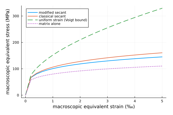

The curves are in the order the theory predicts:

• both estimates lie between the matrix alone and the Voigt bound;

• the modified secant estimate lies below the classical one, because the second moment of the strain is never below the strain of the average, and the matrix softens as its strain grows.

The bound is far above both estimates. Uniform strain forces the strong particles to deform as much as the matrix, whereas in the composite the particles strain much less.

The strains of the phases

The effective strains are the internal variables of the law, named after the phases:

plot(r_mod[:ε11] * 1e3, [r_mod[:M] r_mod[:P]] * 1e3; lw = 2,
    label = ["matrix, modified" "particles, modified"],
    xlabel = "macroscopic equivalent strain (‰)", ylabel = "effective strain of the phase (‰)",
    legend = :topleft)
plot!(r_cla[:ε11] * 1e3, [r_cla[:M] r_cla[:P]] * 1e3; lw = 2, ls = :dash,
    label = ["matrix, classical" "particles, classical"])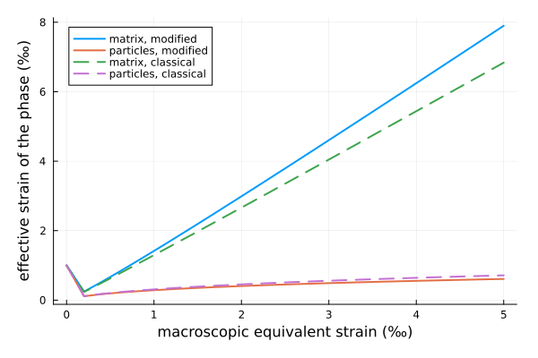

At the end of the path, in ‰:

map(x -> round(1e3 * x; digits = 2), (matrix_modified = r_mod[:M][end], matrix_classical = r_cla[:M][end], macroscopic = e_max))

(matrix_modified = 7.9, matrix_classical = 6.84, macroscopic = 5.0)

The matrix takes most of the deformation, more than the macroscopic strain itself. Its second moment exceeds its average, which is the fluctuation the classical method does not see.

Checks

Linear phases give back the linear scheme. With   a power law is linear elasticity of shear modulus . The secant moduli are then constant, the fixed point is trivial, and the tangent of the composite must be the Mori–Tanaka stiffness itself:

linear(μ, k) = PowerLawElasticity(; k, σ₀ = 3μ * 1e-3, ε₀ = 1e-3, m = 1.0)
rve_lin = RVE()
add_phase!(rve_lin, :M, Ellipsoid(1.0), Dict(:C => TensISO{3}(3 * 60e3, 2 * 20e3)); fraction = :rest)
add_phase!(rve_lin, :P, Ellipsoid(1.0), Dict(:C => TensISO{3}(3 * 150e3, 2 * 80e3)); fraction = f)
h = NonlinearHomogenized(rve_lin, Dict(:M => linear(20e3, 60e3), :P => linear(80e3, 150e3)))
E = Mandel{Float64}(1e-3, 2e-4, -3e-4, 1e-4, 0, 2e-4)
σ, 𝕂, _ = point_update(h, E, initial_state(h), 0.0)
𝕂 ≈ KM(homogenize(rve_lin, MoriTanaka(), :C))

true

The tangent is consistent. The contract checker compares the tangent from the implicit-function theorem with the derivative of the stress:

check_material_interface(modified; verbose = false)

true

Going further

• Any linear scheme can replace Mori–Tanaka, for example NonlinearHomogenized(rve, laws; scheme = SelfConsistent()), with the assumptions on the microstructure that the scheme carries.

• The composite is a law like any other. It runs at the quadrature points of a structure in the same way as the law of the finite-element quickstart.

---

This page was generated using Literate.jl.