The strength of a porous plastic solid

The whole page as one script

Every block of this page, in order, is scripts/material_laws/17_strength.jl. From a clone of the repository, julia --project=docs -e 'using Pkg; Pkg.instantiate()' once, then julia scripts/material_laws/17_strength.jl, runs it end to end.

A porous solid whose solid phase obeys a von Mises criterion has a macroscopic strength domain: the set of macroscopic stresses it can carry. The tutorial From derivatives to a strength criterion builds that domain from the derivatives of the linear effective moduli. This page shows that the same domain is what the secant homogenization of NonlinearHomogenized gives, when the solid is a rigid–perfectly plastic phase law. The approach is that of Barthélémy and Dormieux (2003); the example below runs it.

The solid as a phase law

The solid can carry any stress whose deviator has a norm   at most (no factor under the root, see Conventions). In the deformation theory of plasticity, a rigid–perfectly plastic solid is the power law of PowerLawElasticity with the exponent  : its deviatoric stress has the norm whatever the deviatoric strain, and its secant shear modulus is

Two measures of the same bound must not be confused. This page bounds the norm of the stress deviator,  . The law PowerLawElasticity is written instead with the von Mises stress    and the equivalent strain   , and its parameter σ₀ is a von Mises stress. A solid that bounds by is therefore the law with σ₀ = sqrt(3/2) * σo, as in the example. A positive exponent gives a hardening solid whose response tends to the rigid–plastic one as  . Plastic flow conserves the volume: the solid is given a bulk modulus large against its secant shear modulus.

The secant estimate is a strength

With the modified secant method, the solid takes the secant modulus at the quadratic mean of its deviatoric strain in the linear comparison composite,   . The quadratic mean of its deviatoric stress is then exactly the bound:

Multiply the macroscopic strain by  . The strains of the comparison composite scale by , the secant modulus by , and so does the effective stiffness of a composite of an incompressible solid and empty pores, which is proportional to the shear modulus of the solid. The macroscopic stress    does not change: the composite flows at a constant stress, which is a point of its strength domain. Sweeping the direction of sweeps the boundary of the domain.

The condition   is the one that the tutorial writes with the derivatives of and with respect to the shear modulus of the solid. For an isotropic composite it reads

with the mean stress, the norm of the macroscopic stress deviator and the porosity. For spherical pores and the Mori–Tanaka scheme it becomes the ellipse        . The two routes compute the same domain by different means: the tutorial from two derivatives of the linear moduli, NonlinearHomogenized by solving the secant fixed point at a given strain. Running the phase law brings what the closed construction does not: the direction of flow at each point of the domain, the whole loading path, and any phase law in place of the rigid–plastic one.

Normality

At a point of the boundary, the macroscopic strain that produced it is along the outward normal to the domain: the macroscopic flow obeys the normality rule. The modified secant method coincides with the variational estimate of Ponte Castañeda (1991) for these phases (Suquet, 1997), whose macroscopic potential, in the rigid–plastic limit, is homogeneous of degree one in the strain; its gradient is a stress of the boundary, normal to the direction of the strain. The tests of the package check the normality on the ellipse.

Numerical notes

incompressibility	the bulk modulus of the solid must be large against its secant shear modulus, ; the error on the domain is of the order of their ratio
conditioning	the residual of the fixed point is then accurate to about  , with the machine precision: the tolerance of LocalNewton must stay above it (reltol = 1e-8 for a ratio of )
iterative schemes	with a self-consistent scheme, the tolerance of the local Newton iteration must also stay above that of the scheme's own fixed point
scope	a von Mises solid. A frictional (Drucker–Prager) solid also needs the second moment of the mean strain, as in Maghous et al. (2009); it is not covered

Example: the strength of a porous plastic solid

This example obtains the macroscopic strength domain of a porous solid by running the secant homogenization of a phase law. It compares the result with the closed-form ellipse of Mori–Tanaka and with the construction of the tutorial From derivatives to a strength criterion.

The porous solid

The solid fills 85 % of the volume; the pores are spheres. The solid bounds the norm of its stress deviator by , its strength in units of which every stress below is given:

using MeanFieldHomogenization, TensND, Plots

φ, σo = 0.15, 1.0
rve = RVE()
add_phase!(rve, :S, Ellipsoid(1.0), Dict(:C => TensISO{3}(1.0, 1.0)); fraction = :rest)
add_phase!(rve, :P, Ellipsoid(1.0), Dict(:C => TensISO{3}(1e-12, 1e-12)); fraction = φ)
solid(m) = PowerLawElasticity(; k = 1e6, σ₀ = sqrt(3 / 2) * σo, ε₀ = 1.0, m)

code	theory
:P	the pores, a phase without a law: a linear stiffness close to zero
solid(m)	the solid: a power law of exponent m, rigid–perfectly plastic for m = 0
σ₀ = sqrt(3 / 2) * σo	the von Mises stress of the law, for a bound on
k = 1e6	a bulk modulus large against the secant shear modulus: plastic flow conserves the volume

From hardening to flow

Under a deviatoric macroscopic strain, a hardening solid ( ) makes the composite harden, and the rigid–plastic solid ( ) makes it flow at a constant stress:

dev = LoadingPath(range(0, 1; length = 21); ε11 = t -> 2.0 * t, ε22 = t -> -t, ε33 = t -> -t,
    ε23 = 0, ε13 = 0, ε12 = 0)
p = plot(; xlabel = "macroscopic strain E₁₁", ylabel = "Σ_d / σo", legend = :bottomright)
for m in (0.2, 0.05, 0.0)
    r = point_response(NonlinearHomogenized(rve, Dict(:S => solid(m))), dev; algorithm = LocalNewton(; reltol = 1e-8))
    Σd = [sqrt(2 / 3) * abs(r[:σ11][i] - r[:σ22][i]) for i in eachindex(r.t)]
    plot!(p, r[:ε11][2:end], Σd[2:end] / σo; lw = 2, label = "m = $m")
end
p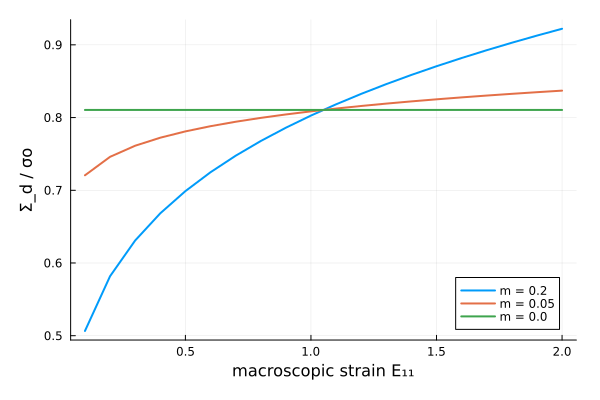

The strains are large because the solid is rigid until it flows: in this limit only the direction of the strain matters, not its size. The tolerance of the local Newton iteration is looser than the default: as the strain grows, the secant shear modulus of the solid falls against its bulk modulus, and the fixed point loses accuracy in proportion (see the numerical notes).

The strength domain

Each direction of the macroscopic strain, from pure expansion to pure contraction through pure shear, gives a point of the boundary of the domain:

𝟏 = Mandel{Float64}(1, 1, 1, 0, 0, 0)
shear = Mandel{Float64}(1, -0.5, -0.5, 0, 0, 0)
mean_dev(σ) = (m = sum(σ[1:3]) / 3; (m, sqrt(sum(abs2, σ - m * 𝟏))))
function domain(h; algorithm = LocalNewton(; reltol = 1e-8))   # see the numerical notes
    pts = map(range(-π / 2 + 0.01, π / 2 - 0.01; length = 41)) do θ
        E = sin(θ) * 𝟏 / 3 + cos(θ) * shear
        mean_dev(point_update(h, E, initial_state(h), 0.0; algorithm)[1])
    end
    return first.(pts), last.(pts)
end
Σm, Σd = domain(NonlinearHomogenized(rve, Dict(:S => solid(0.0))))
θ = range(0, π; length = 200)
a, b = (1 - φ) * σo / sqrt(1.5φ), (1 - φ) * σo / sqrt(1 + 2φ / 3)      # semi-axes of the ellipse
plot(a * cos.(θ), b * sin.(θ); lw = 2, label = "closed-form ellipse (Mori–Tanaka)",
    xlabel = "Σ_m / σo", ylabel = "Σ_d / σo", aspect_ratio = :equal, legend = :outerright, size = (760, 360))
scatter!(Σm, Σd; ms = 3, label = "NonlinearHomogenized, m = 0")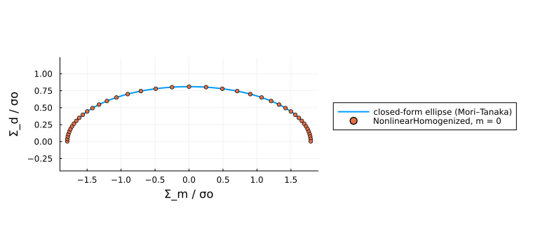

The points of the phase law fall on the ellipse. The mean stress reaches far larger values than the deviatoric one: a hydrostatic stress can only make the porous solid flow by closing or opening its pores.

Another scheme, another shape of pores

With flat spheroidal pores and solid grains of all orientations, and the self-consistent scheme, the domain shrinks sharply. The construction of the tutorial, from the derivatives of the linear moduli, gives the ellipse to compare with:

ω = 0.1
scheme = SelfConsistent(; abstol = 1e-12, maxiters = 500)
function grains(μ_s::T) where {T}
    r = RVE(; T = T, distribution_shape = Ellipsoid(1.0))
    add_phase!(r, :S, Spheroid(ω), Dict(:C => iso_stiffness(convert(T, 1e6), μ_s)); fraction = :rest, symmetrize = IsoSymmetrize())
    add_phase!(r, :P, Spheroid(ω), Dict(:C => iso_stiffness(convert(T, 1e-12), convert(T, 1e-12))); fraction = convert(T, φ), symmetrize = IsoSymmetrize())
    return r
end
using ForwardDiff
kμ(μ) = [k_mu(best_fit_iso(homogenize(grains(μ), scheme, :C)))...]
k, μ = kμ(1.0)
dk, dμ = ForwardDiff.derivative(kμ, 1.0)
A, B = dk / k^2, dμ / μ^2
a_sc, b_sc = sqrt((1 - φ) / (2A)) * σo, sqrt((1 - φ) / B) * σo
Σm_sc, Σd_sc = domain(NonlinearHomogenized(grains(1.0), Dict(:S => solid(0.0)); scheme); algorithm = LocalNewton(; reltol = 1e-9))
plot(a_sc * cos.(θ), b_sc * sin.(θ); lw = 2, label = "derivative construction",
    xlabel = "Σ_m / σo", ylabel = "Σ_d / σo", aspect_ratio = :equal, legend = :outerright, size = (760, 360))
scatter!(Σm_sc, Σd_sc; ms = 3, label = "NonlinearHomogenized, m = 0")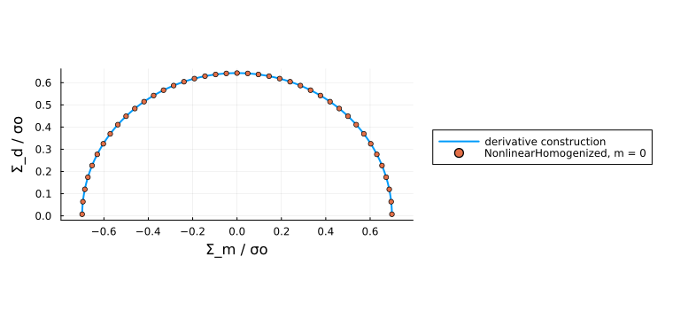

The two routes agree here too. The tolerance of the local Newton iteration is looser still, so as to stay above that of the self-consistent fixed point it contains.

Going further

• A hardening solid ( ), or any law of the strain alone, replaces the rigid–plastic one with no other change, and the composite runs at the quadrature points of a finite-element computation.

• The solid can carry a second phase, rigid or elastic, given as a phase without a law: the domain then accounts for it through the scheme.

---

This page was generated using Literate.jl.