Hill polarization tensors

Before this page

The Eshelby inclusion problem, which defines and the Eshelby tensor, and the Walpole basis and ellipsoid geometry of the Conventions, in which every closed form below is written.

The Eshelby problem reduces to computing one object, the Hill polarization tensor . This page gives its closed forms.

The structure to keep in mind: factors into a purely geometric part, which depends on the ellipsoid alone, and a purely material part, which depends on the reference moduli alone. The geometric part is a set of Newton-potential integrals; every shape — triaxial ellipsoid, spheroid, sphere, infinite cylinder — is one column of the same two tables.

This page follows the appendix Hill polarization tensors of the Echoes manual; expressions, conventions and bibliography are aligned on it. Extensions specific to MeanFieldHomogenization are flagged as such.

Those columns are the shapes below — meridian sections, drawn to scale from the semi-axes each closed form is written in. Every one of them is a limit of the same triaxial ellipsoid, reached by sending an aspect ratio to 1, 0 or ∞: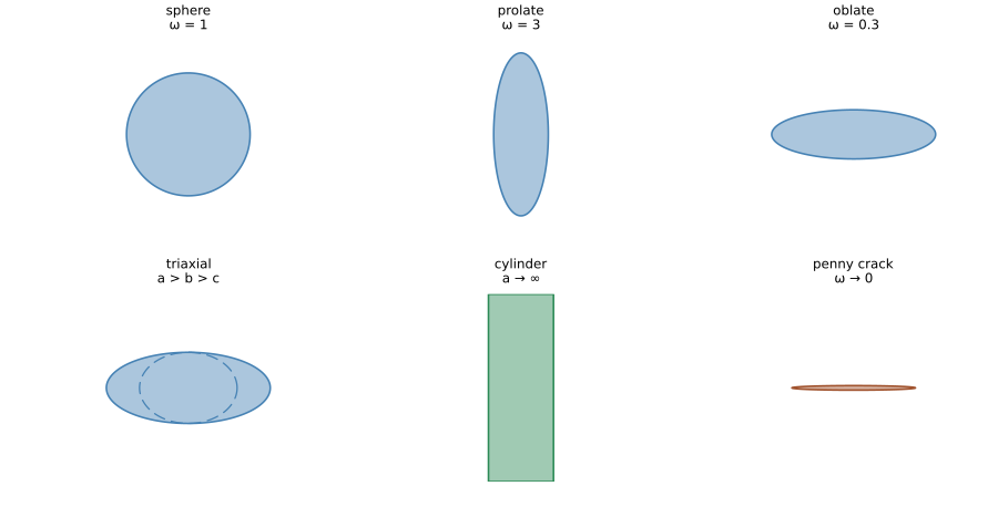

Two of the six are limits rather than bounded bodies: the cylinder leaves the panel because it is unbounded along its axis, and the penny crack is flat rather than thin. The dashed outline in the triaxial panel is the second principal section — the case where no two semi-axes coincide, and the only one that needs the general cubature.

The ribbon crack is deliberately absent: it is the   limit of the penny crack, so in a meridian section it draws exactly the same flat segment. What distinguishes it lies in the crack plane, which this view cannot show — hence the separate RibbonCrack type, and the   column of every table below.

The flat limits are the ones that need care: stays finite there, but the object built on it, , degenerates in a controlled way — which is why the crack theory is written on (Crack opening displacement).

1. Newton-potential integrals

Three integrals over the unit sphere, depending on only, factor every analytical Hill formula:

The two parametrizations of are related by the bijection of the unit sphere onto itself     , whose surface-element identity is

An intrinsic proof is given in Barthélémy et al. (2016), as an alternative to the component reasoning of Mura (1987).

Proof of the surface-element identity

Let   . Differentiating    along the sphere, the variation of only adds a component along :

The map is therefore the linear map followed by the orthogonal projection onto the plane tangent to the sphere at . A linear map carries an oriented surface element to    (Nanson's formula), and the projection onto a plane keeps the component of a surface vector along the normal to that plane. On the two unit spheres    and   , so that, being symmetric,

because      . The inverse map     gives   , which turns the last expression into the identity above.

Both forms are useful: the form makes the geometry explicit, the form is the one that degenerates cleanly in the cylinder limit below.

In MeanFieldHomogenization these are tens_IA, tens_UA and tens_VA.

Principal coefficients

and share their eigenvectors, so

The coefficients , identified with Newton-potential integrals (Kellogg, 1929; Eshelby, 1957; Parnell, 2016), and the secondary coefficients admit closed forms in every symmetry class:

	ellipsoid	prolate spheroid	oblate spheroid	sphere	cylinder

Here   and   are the incomplete elliptic integrals of the first and second kind (Abramowitz and Stegun, 1972),

of amplitude and modulus

The secondary coefficients follow from the by

except where the denominator degenerates — each symmetry class then has its own regular expression:

	ellipsoid	prolate spheroid	oblate spheroid	sphere	cylinder

with  . The circular cylinder   gives    and    .

Normalization differs from the classical references

For writing convenience the coefficients tabulated above are rescaled relative to Kellogg (1929) and Eshelby (1957): they differ by a factor for with  , and by for all the others. The normalization used here is the one that makes  .

Internally, newton_potential_3d and newton_potential_3d_cylinder return the raw kernel — the values above multiplied by — and the division is applied at the tens_IA call site.

Close to a sphere, close to a spheroid

The divided differences of the table, such as    , cancel when two semi-axes come together. newton_potential_3d evaluates them otherwise: a spheroid, sphere included, through the integrals these potentials stand for, and a triaxial ellipsoid whose two semi-axes differ by less than 2 % through an expansion around the spheroid it is close to, exact and differentiable where the two meet. Degenerate shapes gives both.

Why the cylinder column has zeros that still matter

The cylinder column is the limit   of the triaxial one. Three entries vanish, but they carry finite products that survive:

These products appear only through terms ( ) in , where they produce the vanishing first row and column of below and keep the third Eshelby identity valid at the cylinder endpoint. The circular sub-case   is evaluated on a separate branch, avoiding the   intermediates.

Identities

Always satisfied, and useful as numerical checks (Eshelby, 1957):

Components of and

Both are orthotropic along the ellipsoid axes. In the principal frame (Barthélémy et al., 2016; Barthélémy, 2020):

The two tensors as 6×6 Kelvin–Mandel matrices

In the frame , with   and the components ordered , the formulas above fill

the superscript being dropped. The shear entries are twice the tensor components,  ,  , as Kelvin–Mandel storage requires. Substituting the cylinder column of the tables, with the finite limits of the products noted above, gives the two matrices of the cylinder below.

Sphere  :

Infinite elliptic cylinder  , axis , transverse semi-axes   (Mura, 1987; §11.22) — substituting the cylinder column above:

in Kelvin–Mandel storage and in the frame . The vanishing first row and column is the signature of the infinite cylinder: no polarization is transmitted along its axis. For the circular cylinder   the non-zero entries reduce to   ,  ,  , and to the diagonal .

2. Hill tensor in elasticity

Arbitrary anisotropy

This is the form of Willis (1977); see also Mura (1987).

Properties

Scaling by   multiplies and   by the same : depends on the shape of the inclusion through two aspect ratios and the orientation of its axes, not on its size.

is major-symmetric and positive definite on symmetric second-order tensors, for any positive definite . The Eshelby tensor    is not major-symmetric in general. It is similar to   , so its eigenvalues are real and positive; being non-symmetric, its quadratic form is not controlled by them. The stress counterpart      is defined in The Eshelby inclusion problem.

Why ℙ is positive definite

For a symmetric and a symmetric ,          . Hence, from the form,

The acoustic tensor is symmetric positive definite, since            for  , and so is its inverse. The integrand is therefore non-negative, and the integral, of a continuous integrand, vanishes only if    for every unit , that is  .

Reduction to a sphere

Every ellipsoid can be described by a symmetric positive definite    , its semi-axes and their orientation. In the form above, the shape then enters only through the vector  , and pulling out of the integral moves it onto the stiffness: the integrand becomes that of a sphere in the medium

which the affine stretch mapping the ellipsoid onto the unit ball makes of . The Hill tensor of the ellipsoid follows from that of the sphere by the same tensor on each side (Barthélémy, 2020; eq. 8):

The same reduction was reached by Pouya (2000), Pouya and Zaoui (2006) from the field equations. It has two uses. A numerical method need only treat the sphere, where the denominator   of the form is one. And a family of matrices that the stretch maps onto one whose spherical Hill tensor is known inherits a closed form: an elliptically orthotropic matrix       maps onto an isotropic one (Barthélémy, 2020; eq. 14), and a transversely isotropic matrix coaxial with a spheroid stays transversely isotropic, which gives the closed form of the section below. The tutorial Hill tensors by reduction to a sphere computes several Hill tensors both ways, and the application Hill tensors by transformation derives the reduction, and its elliptically orthotropic case, step by step after the paper.

Algorithms for an arbitrary anisotropy

Inverting the acoustic tensor    pointwise is the source of all the computational work: in general no closed form exists and one resorts to numerical integration (Ghahremani, 1977; Gavazzi and Lagoudas, 1990; Masson, 2008). MeanFieldHomogenization offers three algorithm traits, mirroring the Echoes NUMINT / RESIDUES options:

• NestedQuadGK — nested adaptive 1-D Gauss–Kronrod quadratures, type-generic and always available, the :auto choice whatever the coefficient type and whatever else is loaded.

• DECUHR — the surface integral is evaluated by the adaptive cubature for singular integrands of Espelid and Genz (1994). ForwardDiff-safe, on an explicit method = :decuhr once its (weak-dependency) extension is loaded.

• Residue — the inner integral is reduced to a sum of residues at the roots of the acoustic polynomial by the Cauchy theorem, leaving a single 1-D quadrature (Masson, 2008). With the substitution   of that paper, the inner integral is that of a rational function of over , which is minus the sum of the residues of its product with . Roots that coincide or nearly do, as for an isotropic or transversely isotropic reference along the ellipsoid axes or a reference close to one, are summed as a group (below), so that the sum keeps the accuracy of separated roots. The method is Float64-only (the roots are the eigenvalues of a companion matrix, which ForwardDiff does not differentiate) and reachable on an explicit method = :residues only.

The residue algorithm is the one whose accuracy depends most on how it is evaluated; the next section derives it in full.

Residue sums over groups of poles

The inner integral as a rational one. At an angle of the outer quadrature, the directions of integration form the line    ,  , and the inner integral is a combination of the seven moments

where     is the acoustic polynomial, of degree 6, positive on the real line for a strongly elliptic matrix, and the power comes from the normalization of the direction. That power puts branch points at   , which a residue theorem cannot take as they are. The substitution of Masson (2008),   , removes them:   maps onto with    , and

a rational function whose denominator, of degree 16, has the double roots   , the images of the branch points, and the two preimages    of each root of , the roots of    , whose product is .

Proof of the change of variable

With   ,    , so that increases from to on , and     for  . Then

and multiplying above and below by gives , since    and is a polynomial in .

The integral over a half line. For a rational   with    and no root of on ,

the sum running over all the roots of , with the logarithm cut along the positive axis,  . This is the argument of Masson (2008), eqs. 17–19, who integrates the product of with a logarithm along a keyhole contour (his Fig. 2) and writes the sum for simple roots of , with formulas of their own for a root at and for roots that coincide (his eqs. 21–22 and those after), the case of two roots at being left open. The sums over groups of poles below take every one of these cases, and the roots that nearly coincide, in one formula. As has real coefficients its roots come in conjugate pairs, and the sum reduces to the upper half plane:

Proof

Integrate along the keyhole contour made of the circle  , the circle   and both edges of the cut . On the large circle the integrand is and the circle has length : its contribution vanishes as  , and so does that of the small one, , as  . On the upper edge  , on the lower one   , run in the opposite direction, so that the two edges give      . The residue theorem gives , whence the first formula.

For the second,   gives  , and with the cut along the positive axis    for   , an identity between functions analytic near , which holds for poles of any multiplicity:    . Adding the residues at and leaves      , and the integral, real, keeps the real part,    .

The sum over a group of close poles. A root of multiplicity comes out of any root finder as roots about apart, the unit roundoff, and the residue at each is of the order of the inverse of their distance. Taken one by one, the residues are large, of opposite signs, and their sum keeps little of their accuracy; declared coincident below some distance, they carry an error of the order of that distance. The residues of a group are summed as a whole instead.

Let be poles of close to one another, with and polynomials and analytic around them (  or  ), their centroid,   ,  ,   , which does not vanish near , and the distance from to the nearest singularity of : the other roots of and, for  , the branch point . For  ,

with the complete homogeneous symmetric polynomial of degree , the sum of all the monomials of degree in the .

Proof, and the rate of the series

The sum of the residues in the group is along the circle     with   . On ,    and

the product of geometric series, uniformly convergent on ; the Taylor series of converges uniformly there too, as  . The integral of the product picks the coefficient of  , that is the terms     .

Coincident poles leave the term   alone, , the residue at a pole of order ; a lone pole leaves  . As   and, by the Cauchy estimates on a circle of radius  ,  , the terms decrease as : the series converges geometrically at the rate , and the poles enter through symmetric functions of the only, which, unlike the individual roots of a cluster, are well conditioned: they are, up to sign, the coefficients of   , which the root finder returns accurate to rounding.

The sum is evaluated by recurrences of fixed cost. The follow from multiplying the geometric series one at a time,   . The Taylor coefficients of follow from dividing by each factor     in turn,    , those of from     , and those of from its factored form. The series is cut at the first with below the unit roundoff. The groups are the largest nodes of the single-linkage tree of the poles whose ratio stays below , each pole going to the largest node that qualifies; a lone pole is a group of one. A tree is needed: four roots spread around a double pole, as a double root of at gives, form a tight group of six that no pair, and no group of three, qualifies to start.

Conditioning, and the running error bound. The sums above are exact, but their evaluation is not always well conditioned. When a root of approaches , as it does for the directions of a plane of isotropy of the matrix (around a sphere in an isotropic matrix,   ), its preimages approach the double pole  , at the distance . Poles then crowd around at several scales: groups of radius comparable to their distance to the others, or to the branch point , cannot be merged into one whose series converges, and their contributions are larger than their sum by four or five orders of magnitude. The integral itself stays as well conditioned as anywhere else: only its representation by residues is not.

Each sum therefore carries a running error bound. The same recurrences are run on the moduli of their operands, every difference turned into a sum; the result bounds, term by term, the moduli of the quantities each step adds up, and the rounding error of the sum is at most a small multiple of the unit roundoff times that bound (Higham, 2002). Against the same sums in 256-bit arithmetic, on groups from a lone pole to an eightfold one, the error stayed below the bound times the unit roundoff by a factor 2.8 at least; the package takes four times that product. When the bound exceeds the tolerance asked of the inner integral, an order and more below that of the outer quadrature, the moments are computed by an adaptive Gauss-Kronrod quadrature of their definition in instead, which is accurate there. A spheroid elongated along the axis of a transversely isotropic matrix, at a relative tolerance of , met such directions over a whole range of : evaluated anyway, the sums were off and kept the outer quadrature from converging, a million evaluations and 35 s for one tensor; with the bound, it takes 285 evaluations and 0.02 s, within   of the closed form.

For the line integral of the crack opening tensor,   and the poles are the roots of themselves: the same groups, the same bound, and the quadrature of the same kernel when the bound exceeds the tolerance.

All three honor the abstol (default ), reltol () and maxiters ( evaluations) keywords of hill_tensor. At these defaults NestedQuadGK is within about of the exact value — of a closed form where one exists, of a tight reference checked by a second algorithm otherwise — and DECUHR within to ; on a triaxial ellipsoid    in a triclinic matrix NestedQuadGK takes about 1 ms, the residues and DECUHR about 4 ms (Performance vs Echoes).

Flat ellipsoids,   , are a case apart. The integrand is regular there, so DECUHR runs as an adaptive Gauss rule; it gives the values of the Echoes NUMINT3D option at equal tolerances. At the default tolerances its error is to   at   and . At tolerances it is still   at  , for about 0.5 s per tensor. NestedQuadGK stretches the end   of its outer interval by    , with   . The integrand also varies over a layer   at the other end, so below   breakpoints at     give that layer intervals of its own. The result then stays within the tolerance asked for down to  : at most   at the defaults, and   at in 2 to 4 ms.

Analytical paths exist in the literature for further anisotropy classes (Withers, 1989; Pouya, 2000; Pouya and Zaoui, 2006; Suvorov and Dvorak, 2002) and are not all implemented yet.

Isotropic matrix — the shape/moduli factorization

With bulk modulus , shear modulus and first Lamé parameter   , so that         , the general expression collapses to the form of Willis (1977)

This is the factorization announced at the top of the page: shape and orientation on one side (, ), reference moduli on the other. Each shape column of the tables above therefore yields a closed-form at once.

For a sphere, substituting and gives the classical Eshelby result

For an infinite cylinder, substituting and gives a closed form with  , i.e. no polarization along the axis (Mura, 1987; §11.22).

Implementation: src/Elasticity/hill_3d_iso.jl and src/Elasticity/hill_3d_cylinder_iso.jl, selected by method = :auto when is a TensISO.

Transversely isotropic matrix coaxial with a spheroid

Let the spheroid have its axis along and the aspect ratio (axial over transverse semi-axis), so that ``\boldsymbol{A} = \underline{e}_1\otimes\underline{e}_1 + \underline{e}_2\otimes\underline{e}_2

• \omega,\underline{e}_3\otimes\underline{e}_3`` up to a scale, and let the

matrix be transversely isotropic about the same axis, with the five constants . The stretch of the reduction to a sphere divides each component of by to the number of its indices equal to 3: the transformed matrix is still transversely isotropic, and so are the Hill tensors of the sphere in it and of the spheroid in (Barthélémy, 2020; eqs. 18–20). The latter has five Walpole coefficients (see Conventions):

The sphere in a transversely isotropic medium has a closed form (Barthélémy, 2020; eqs. 24–29), and carried back through the stretch it gives the spheroid (Barthélémy, 2020; eqs. 30–36). The derivation goes in three steps, each of them carried out on free symbols in the application Hill tensors by transformation.

Derivation: the sphere in the transformed medium, then the spheroid

The transformed medium. With        , is transversely isotropic about , of constants  ,  ,  ,   and  , and the Walpole coefficients of are those of   divided by , , , and .

The sphere. On the unit sphere, in the colatitude and the longitude with  , is the average of   ,    . Medium and directions are invariant by the rotations about , so that the integrand at is that at   rotated, and its average over is the projection of the integrand at   on the Walpole basis: the integral over costs nothing. At   the acoustic tensor has the components

over the two denominators       and    , where are the roots of the acoustic polynomial written with the constants of and   . Each projected coefficient is then an even polynomial in over or , and the integral over    is a combination of

 , which are the integrals and of Degenerate shapes.

Back to the spheroid. Substituting for the unknown divides the acoustic polynomial of by , which turns it into that of :  , and likewise  . Writing the constants of in those of and dividing by the powers of above gives the coefficients below.

The acoustic parameters of the matrix are the square roots of the two roots of

taken with a positive real part. As is positive definite, and are either both real and positive or complex conjugates, so that everything below is real. With   and  , the Walpole coefficients are

A sphere is coaxial with every axis: at   these are the coefficients of a sphere in a transversely isotropic matrix, those of the transformed problem above with   (Barthélémy, 2020; eq. 29). A sphere in a TensTI matrix therefore takes this closed form whatever the axis of the matrix, with no quadrature.

As written, the coefficients cancel near the sphere, at coincident roots (an isotropic matrix stored as transversely isotropic), for a disc and for a needle, and a square root of zero spoils the derivatives at an isotropic point. Degenerate shapes rewrites them in a form that stays exact to rounding everywhere, derivatives included, and that is the form the package evaluates; the application transcribes the formulas as written, and measures what they lose (The script of the paper, in Julia).

Flat and needle limits. As   the spheroid flattens into a penny-shaped crack and     , with      , of Walpole coefficients and on and , and in closed form in (Barthélémy, 2020; eqs. 37–39). The crack compliance   , with      the second Hill tensor (second_hill_tensor), depends on only and has two Walpole coefficients (Barthélémy, 2020; eqs. 40–41):

the transversely isotropic case of the crack opening tensors of COD tensors. As   the spheroid tends to a circular cylinder and  ,    ,  ,  , with corrections in (Barthélémy, 2020; eq. 42). The expansions are derived symbolically, and held to the package, in The flat spheroid and the crack and The needle.

The dispatcher routes a TensTI{4} matrix combined with a coaxial Ellipsoid{3, Spherical|Prolate|Oblate} to this path by default; coaxiality is detected by _ti_coaxial(C₀, ell). Non-coaxial spheroids and triaxial ellipsoids fall back to the anisotropic default, i.e. a cubature. Implementation: src/Elasticity/hill_3d_ti_coaxial.jl.

Anisotropic matrix, cylinder limit

Cylinder is a first-class inclusion type here (extension over Echoes). For an arbitrarily anisotropic matrix the residue algorithm does not apply: it rests on the six complex roots of the acoustic polynomial along , and at the cylinder limit one root escapes to infinity, degenerating the polynomial.

The form of the Willis integral degenerates cleanly instead. The axial component of vanishes identically, so the surface integral collapses to a single quadrature over the transverse unit circle:

This is a one-dimensional QuadGK integral, and it stays ForwardDiff-compatible. Calling hill_tensor(Cylinder(…), C₀; method = :residues) falls back to it silently. Implementation: src/Elasticity/hill_3d_cylinder_aniso.jl (CylinderQuadrature trait). The in-plane components coincide with the solution of the 2-D plane-strain problem — the cylinder is the 3-D realization of the 2-D ellipse.

2-D plane strain

Plane strain is handled directly (extension over Echoes), integrating over the unit circle   with a prefactor in place of . The isotropic case is analytical; the anisotropic one uses the residue reduction on the line integral.

3. Hill tensor in conductivity

The order-2 Hill tensor of the transport problem, defined in The Eshelby inclusion problem §3, is built on the same integral of §1 and, unlike its elastic counterpart, has a closed form at any anisotropy of the reference medium.

Arbitrary anisotropy — closed form

For a conductivity tensor (Willis, 1977):

Unlike the order-4 case, this integral has a closed form for any matrix anisotropy. Since is symmetric positive definite it has a square root,    , and the denominator can be absorbed into the change of variable    , which turns the anisotropic problem into an isotropic one for a fictitious ellipsoid of shape tensor  :

This is the transformation derivation of Giraud et al. (2019); an equivalent Green's-function derivation is given in Barthélémy (2009). Since   need not be symmetric, the fictitious semi-axes and principal directions are obtained by diagonalizing    .

Isotropic matrix — immediate

If    the prefactor comes straight out:

For a sphere,   gives   and   — independent of . Implementation: src/Conductivity/hill_order2_3d.jl.

4. Dispatch

The closed forms above are reached through one entry point, which selects the algorithm from the inclusion type and from the type of the reference tensor.

Entry point hill_tensor; shape tensor via shape_tensor; geometric auxiliaries via tens_IA, tens_UA, tens_VA.

(inclusion, C₀)	:auto selects	alternatives	ForwardDiff
Ellipsoid{3}, TensISO	Analytical	—	✓
Ellipsoid{3}, TensTI (coaxial)	Analytical (MFH)	:residues, :decuhr	✓
Ellipsoid{3}, AbstractTens{4,3}	NestedQuadGK	:residues, :decuhr, :nestedquadgk	✓
Cylinder, TensISO	Analytical	—	✓
Cylinder, AbstractTens{4,3}	CylinderQuadrature	(residue degenerates)	✓
Ellipsoid{2}, TensISO	Analytical	—	✓
Ellipsoid{2}, AbstractTens{4,2}	Analytical (residue)	—	(Float64)
Ellipsoid{3}, AbstractTens{2,3}	Analytical ()	—	✓
Cylinder, AbstractTens{2,3}	Analytical	—	✓

Cylinder shape traits: CircularCylindrical when   (transversely isotropic response, returned as TensTI{4} with axis ) and EllipticCylindrical when   (orthotropic, returned as TensOrtho). Practical usage is covered in the manual page Cylindrical inclusions.

Where to go next

The Hill tensor is the response of an inclusion to a prescribed polarization. The next page, Concentration and contribution tensors, turns it into the response of an inhomogeneity to a remote load and into the contribution of each phase to the effective stiffness. The flat limits announced at the top of this page are taken in Crack opening displacement and compliance, and the tutorial Hill polarization tensors in practice evaluates these closed forms and compares the algorithms of §4 on an anisotropic matrix.