Transport properties

Before this page

The tutorial Every scheme on the whole porosity range, whose porous medium and schemes are carried over below to a diffusivity, and the theory page Extension to conductivity, which states the dictionary between the elastic and the transport problems.

Transport properties — diffusivity, permeability, thermal or electrical conductivity — are described by 2nd-order symmetric tensors. They are homogenized with exactly the same machinery as 4th-order elastic properties: only the property key passed to homogenize changes.

Homogenizing a 2nd-order property

A property is stored in each phase under a symbol key — :C for stiffness, :K for conductivity/diffusivity — and selected at homogenization time:

using MeanFieldHomogenization
using TensND
using LinearAlgebra
using Plots
gr()  # headless backend; GKSwstype is set to "100" in make.jl

# Isotropic diffusivities: 2nd-order isotropic tensors.
D_solid = TensISO{3}(0.1)
D_pore = TensISO{3}(1.0)

rve = RVE()
add_phase!(rve, :SOLID, Ellipsoid(1.0, 1.0, 1.0), Dict(:K => D_solid); fraction = :rest)
add_phase!(
    rve, :PORE, Ellipsoid(1.0, 1.0, 0.1), Dict(:K => D_pore);
    fraction = 0.2, symmetrize = IsoSymmetrize()
)

D_eff = homogenize(rve, MoriTanaka(), :K)
tr(Array(D_eff)) / 3

0.19065028014161733

TensISO{3}(k) builds the isotropic 2nd-order tensor  ; note the single argument, against two () for a 4th-order isotropic stiffness.

The scheme is a free parameter, exactly as in elasticity:

for scheme in (Dilute(), MoriTanaka(), SelfConsistent())
    D = homogenize(rve, scheme, :K)
    println(rpad(string(nameof(typeof(scheme))), 16), tr(Array(D)) / 3)
end

Dilute          0.18064276801551857
MoriTanaka      0.19065028014161733
SelfConsistent  0.1994431324590776

The self-consistent estimate sits above Mori-Tanaka here because the conductive pores percolate in the SC topology, while MT keeps them isolated in a continuous, poorly conductive solid.

Diffusivity of a porous medium

The effective diffusivity of a porous material depends strongly on pore shape, not only on porosity. Flat pores (small aspect ratio ) are far more efficient at connecting the medium, per unit volume, than spherical ones.

function D_eff_porous(φ, ω; scheme = SelfConsistent())
    r = RVE()
    add_phase!(r, :CEMENT, Ellipsoid(1.0, 1.0, 1.0), Dict(:K => TensISO{3}(0.1)); fraction = :rest)
    add_phase!(
        r, :PORE, Ellipsoid(1.0, 1.0, ω), Dict(:K => TensISO{3}(1.0));
        fraction = φ, symmetrize = IsoSymmetrize()
    )
    return tr(Array(homogenize(r, scheme, :K))) / 3
end

φs = 0.0:0.15:0.6
println("  φ   ", join(["  ω=$ω" for ω in (0.01, 0.1, 1.0, 10.0)]))
for φ in φs
    vals = [D_eff_porous(φ, ω) for ω in (0.01, 0.1, 1.0, 10.0)]
    println(rpad(φ, 6), join([rpad(round(v, digits = 4), 8) for v in vals]))
end

  φ     ω=0.01  ω=0.1  ω=1.0  ω=10.0
0.0   0.1     0.1     0.1     0.1
0.15  0.186   0.171   0.1457  0.1632
0.3   0.2811  0.2642  0.2261  0.2502
0.45  0.3945  0.3816  0.3503  0.3679
0.6   0.5312  0.5243  0.5084  0.5161

The same sweep, plotted as effective diffusivity against porosity for a range of pore aspect ratios :

φ_plot = 0.0:0.02:0.6
plt = plot(;
    xlabel = "porosity φ", ylabel = "effective diffusivity D_eff",
    legend = :topleft, framestyle = :box, size = (760, 480),
)
for ω in (0.01, 0.1, 1.0, 10.0)
    plot!(plt, φ_plot, [D_eff_porous(φ, ω) for φ in φ_plot]; label = "ω = $ω", lw = 2)
end
plt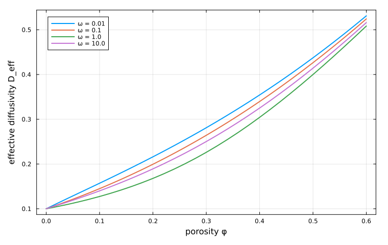

At a given the oblate curve sits well above the others: a thin disc bridges a larger span of the microstructure than a compact inclusion of the same volume.

Two limits are worth checking. At zero porosity every curve must return the solid diffusivity, and at   (spherical pores) the self-consistent estimate must reproduce the classical Bruggeman result — the root of

# Plain bisection — no extra dependency needed.
function bruggeman(φ; Ds = 0.1, Dp = 1.0)
    f(D) = φ * (Dp - D) / (Dp + 2D) + (1 - φ) * (Ds - D) / (Ds + 2D)
    lo, hi = 1.0e-12, 10.0
    for _ in 1:200
        mid = (lo + hi) / 2
        f(lo) * f(mid) <= 0 ? (hi = mid) : (lo = mid)
    end
    return (lo + hi) / 2
end

for φ in (0.2, 0.4, 0.6)
    sc = D_eff_porous(φ, 1.0)
    br = bruggeman(φ)
    println("φ = ", φ, "   SC = ", round(sc, digits = 8),
        "   Bruggeman = ", round(br, digits = 8),
        "   |Δ| = ", round(abs(sc - br), sigdigits = 3))
end

φ = 0.2   SC = 0.16786262   Bruggeman = 0.16786262   |Δ| = 2.27e-10
φ = 0.4   SC = 0.30430749   Bruggeman = 0.30430749   |Δ| = 3.25e-10
φ = 0.6   SC = 0.50835623   Bruggeman = 0.50835623   |Δ| = 2.3e-10

The two agree to  , i.e. to the tolerance of the self-consistent fixed point — a non-trivial check that the 2nd-order SC scheme reproduces the classical effective-medium result for spherical inclusions.

Anisotropy induced by oriented pores

If the pores are not re-oriented isotropically, the effective diffusivity inherits their symmetry. Dropping symmetrize = IsoSymmetrize() leaves all pores aligned on , and the effective tensor becomes transversely isotropic:

r = RVE()
add_phase!(r, :CEMENT, Ellipsoid(1.0, 1.0, 1.0), Dict(:K => TensISO{3}(0.1)); fraction = :rest)
add_phase!(
    r, :PORE, Ellipsoid(1.0, 1.0, 0.05), Dict(:K => TensISO{3}(1.0));
    fraction = 0.15
)

D_aniso = Array(homogenize(r, MoriTanaka(), :K))
(D_11 = D_aniso[1, 1], D_33 = D_aniso[3, 3])

(D_11 = 0.20527498300671992, D_33 = 0.11669699311419938)

The oblate pores lie in the plane, so they short-circuit in-plane transport ( large) while barely helping through-thickness transport ( close to the solid value).

Sweeping the porosity makes the induced anisotropy explicit — the in-plane and through-thickness diagonal components fan apart as grows:

function D_aniso_components(φ; ω = 0.05)
    r = RVE()
    add_phase!(r, :CEMENT, Ellipsoid(1.0, 1.0, 1.0), Dict(:K => TensISO{3}(0.1)); fraction = :rest)
    add_phase!(
        r, :PORE, Ellipsoid(1.0, 1.0, ω), Dict(:K => TensISO{3}(1.0));
        fraction = φ
    )
    D = Array(homogenize(r, MoriTanaka(), :K))
    return D[1, 1], D[3, 3]
end

φ_plot = 0.0:0.01:0.3
D11 = [D_aniso_components(φ)[1] for φ in φ_plot]
D33 = [D_aniso_components(φ)[2] for φ in φ_plot]
plt2 = plot(;
    xlabel = "porosity φ", ylabel = "effective diffusivity",
    legend = :topleft, framestyle = :box, size = (760, 480),
)
plot!(plt2, φ_plot, D11; label = "D₁₁ (in-plane)", lw = 2)
plot!(plt2, φ_plot, D33; label = "D₃₃ (through-thickness)", lw = 2, ls = :dash)
plt2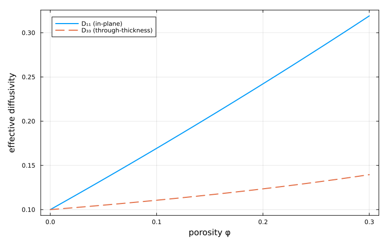

Effect of the Interfacial Transition Zone (ITZ)

The pores considered so far are homogeneous inclusions; the transport schemes accept composite ones as well, of which the aggregate of a mortar is the classical example.

In mortar, the Interfacial Transition Zone is a thin shell (~50 µm) of higher-porosity — hence higher-diffusivity — cement paste around each aggregate. The reduction in diffusivity caused by the impermeable aggregates can be offset, or even reversed, by this more permeable surrounding shell. The morphology is drawn below after the Echoes book (Barthélémy, 2026).

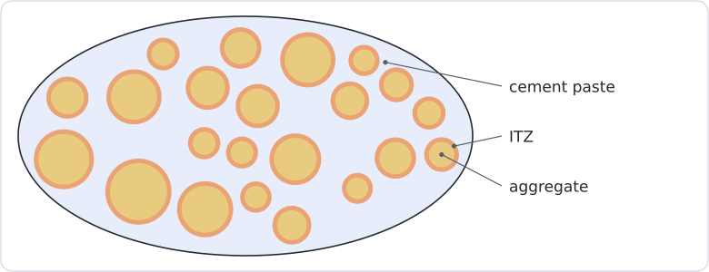
The aggregate + ITZ is a two-layer LayeredSphere — an impermeable core ( , radius ) inside an ITZ shell (thickness ) — embedded in the cement-paste matrix of reference diffusivity   and homogenized by Mori-Tanaka. Because the composite-sphere inclusion covers aggregate and shell, its volume fraction exceeds the bare-aggregate fraction :    .

const Ragg, eITZ = 5.0e3, 50.0    # µm

function D_itz(f, d_itz)
    f_inc = f * (1 + eITZ / Ragg)^3
    r = RVE()
    add_phase!(r, :CEMENT, Ellipsoid(1.0), Dict(:K => TensISO{3}(1.0)); fraction = :rest)
    agg = LayeredSphere((Ragg, Ragg + eITZ), (TensISO{3}(0.0), TensISO{3}(d_itz)))
    add_phase!(r, :AGG, agg, Dict(:K => TensISO{3}(1.0)); fraction = f_inc)
    return tr(Array(homogenize(r, MoriTanaka(), :K))) / 3
end

# spot values reproduce the Echoes reference exactly
[round(D_itz(0.2, d), digits = 4) for d in (0.001, 50.0, 100.0)]

3-element Vector{Float64}:
 0.7198
 0.9979
 1.1604

Sweeping the aggregate fraction for a range of ITZ-to-paste diffusivity ratios , against the two classical bounds for purely impenetrable spheres (  and the Maxwell form   ):

fs = range(0.001, 0.85; length = 40)
plt3 = plot(; xlabel = "aggregate fraction f", ylabel = "D_eff / D_cp",
    legend = :topright, framestyle = :box, ylims = (0, 2), size = (760, 480))
for d in (100.0, 60.0, 50.0, 40.0, 20.0, 0.001)
    lbl = d ≥ 1 ? "D_itz/D_cp = $(Int(d))" : "D_itz/D_cp = 0"
    plot!(plt3, fs, [D_itz(f, d) for f in fs]; lw = 2, label = lbl)
end
plot!(plt3, fs, [(1 - f)^1.5 for f in fs]; c = :black, ls = :dash, label = "(1-f)^{3/2}")
plot!(plt3, fs, [(1 - f) / (1 + 0.5f) for f in fs]; c = :black, ls = :dot, label = "(1-f)/(1+f/2)")
plt3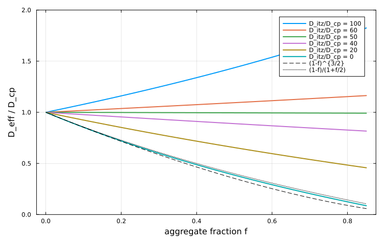

The role of the aggregate + ITZ composite depends strongly on : an impermeable ITZ () drives below both impenetrable-sphere bounds; near   the two effects nearly cancel and  ; a highly permeable ITZ () turns the shells into a connected fast-transport network that lifts above the neat paste value.

Zero-thickness interface (DUALDISC)

In the limit   the thin, highly-conductive ITZ shell can be collapsed onto a zero-thickness surface-conductive interface carrying a tangential surface current    with transmissivity     — the Echoes book's DUALDISC model. This is exactly a SurfaceConductiveInterface on a bare aggregate (a one-layer LayeredSphere); it avoids the explicit shell and its volume-fraction correction   :

function D_dualdisc(f, d_itz)
    α = d_itz * eITZ                                   # transmissivity D_s·e
    agg = LayeredSphere((Ragg,), (TensISO{3}(0.0),);
        interfaces = (SurfaceConductiveInterface(α),))
    r = RVE()
    add_phase!(r, :CEMENT, Ellipsoid(1.0), Dict(:K => TensISO{3}(1.0)); fraction = :rest)
    add_phase!(r, :AGG, agg, Dict(:K => TensISO{3}(1.0)); fraction = f)
    return tr(Array(homogenize(r, MoriTanaka(), :K))) / 3
end

# D_itz/D_cp = 50 makes the surface current exactly offset the impermeable core
[round(D_dualdisc(f, 50.0), digits = 6) for f in (0.1, 0.5, 0.9)]

3-element Vector{Float64}:
 1.0
 1.0
 1.0

The surface-conductive interface reproduces the Echoes DUALDISC diffusivity to machine precision, and agrees with the explicit two-layer model up to the small ITZ volume that the interface idealization neglects:

plt4 = plot(; xlabel = "aggregate fraction f", ylabel = "D_eff / D_cp",
    legend = :topleft, framestyle = :box, ylims = (0, 2), size = (760, 480))
for (d, c) in ((100.0, 1), (50.0, 2), (20.0, 3))
    plot!(plt4, fs, [D_itz(f, d) for f in fs]; lw = 2, c = c,
        label = "layer model — D_itz/D_cp = $(Int(d))")
    plot!(plt4, fs, [D_dualdisc(f, d) for f in fs]; lw = 2, c = c, ls = :dash,
        label = "DUALDISC — D_itz/D_cp = $(Int(d))")
end
plt4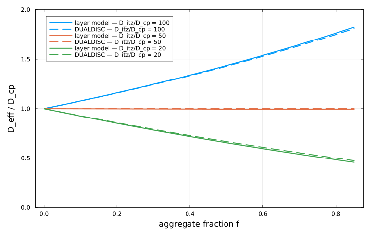

At   the transmissivity   gives an effective sphere conductivity   , so the aggregate becomes transparent and   at every fraction — the flat curve above.

Cross-property coupling

Because a single RVE carries several property keys at once, the same microstructure can be homogenized for stiffness and for transport without being rebuilt — which is the basis of cross-property correlations (Sevostianov and Kachanov, 2002):

r2 = RVE()
add_phase!(r2, :SOLID, Ellipsoid(1.0, 1.0, 1.0), Dict(:C => TensISO{3}(30.0, 12.0), :K => TensISO{3}(0.1)); fraction = :rest)
add_phase!(
    r2, :PORE, Ellipsoid(1.0, 1.0, 0.1),
    Dict(:C => TensISO{3}(1.0e-9, 1.0e-9), :K => TensISO{3}(1.0));
    fraction = 0.15, symmetrize = IsoSymmetrize()
)

C_eff = homogenize(r2, MoriTanaka(), :C)
D_eff2 = homogenize(r2, MoriTanaka(), :K)
(bulk = k_mu(C_eff)[1], diffusivity = tr(Array(D_eff2)) / 3)

(bulk = 4.07913658548325, diffusivity = 0.16594191441863304)

The bulk modulus and the mean diffusivity above come from one microstructure, described once and read twice through the property key.

Where to go next

Every tutorial so far is elastic or conductive, with no dependence on time. Viscoelastic composites opens the extension to viscoelasticity, with complex moduli in the frequency domain and a first aging creep calculation. The order-2 calls of the library are collected in Conductivity of the manual, and Cement paste: chloride diffusivity and elasticity applies the cross-property route of the last section to a hydrating cement paste.