Elastoplastic bar under cycles

The whole page as one script

Every block of this page, in order, is scripts/material_laws/01_plasticity.jl. From a clone of the repository, julia --project=docs -e 'using Pkg; Pkg.instantiate()' once, then julia scripts/material_laws/01_plasticity.jl, runs it end to end.

A steel bar is pulled, pushed back and pulled again. With von Mises plasticity the response depends on how the yield surface hardens: it grows (isotropic hardening) or it moves (kinematic hardening). This example runs both with J2Plasticity, checks the first against its closed form, and shows the difference a reversal makes.

The law and the path

The parameters, in MPa: Young's modulus , Poisson's ratio , the initial yield stress , and a hardening modulus of 10 GPa, given to the isotropic part in one law and to the kinematic part in the other.

using MeanFieldHomogenization, Plots

E, ν, σ₀, h = 200e3, 0.3, 250.0, 10e3
isotropic = J2Plasticity(; E, ν, σ₀, H = h)
kinematic = J2Plasticity(; E, ν, σ₀, Hkin = h)

The path drives the axial strain through a cycle, 0 → 0.4 % → −0.4 % → 0.4 %, the lateral faces being free (every other stress component is zero):

ε_axial(t) = t < 0.25 ? 4e-3 * 4t : t < 0.75 ? 4e-3 * (1 - 4(t - 0.25)) : 4e-3 * (-1 + 4(t - 0.75))
path = LoadingPath(range(0, 1; length = 201); ε11 = ε_axial)
r_iso = point_response(isotropic, path)
r_kin = point_response(kinematic, path)

The first loading against the closed form

In uniaxial stress the elastic part has slope up to , then the slope is  : each increment of strain splits between an elastic part and a plastic part .

first_load = 1:51                      # t ∈ [0, 0.25]
ε = r_iso[:ε11][first_load]
closed_form = [e ≤ σ₀ / E ? E * e : σ₀ + E * h / (E + h) * (e - σ₀ / E) for e in ε]
maximum(abs, r_iso[:σ11][first_load] - closed_form)        # MPa

1.7053025658242404e-13

The two agree to the rounding of the numbers: the backward Euler integration of linear hardening is exact, and the driver finds the free lateral strains to of the stress.

What the reversal shows

plot(r_iso[:ε11] * 100, r_iso[:σ11]; label = "isotropic hardening", lw = 2,
    xlabel = "axial strain ε₁₁ (%)", ylabel = "axial stress σ₁₁ (MPa)", legend = :topleft)
plot!(r_kin[:ε11] * 100, r_kin[:σ11]; label = "kinematic hardening", lw = 2, ls = :dash)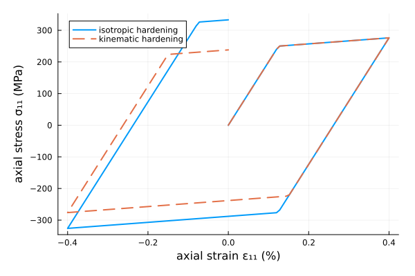

Both laws give the same first loading. On the way back they part:

• with isotropic hardening the yield surface has grown, and the bar must be unloaded by twice its current yield stress before it yields again in compression;

• with kinematic hardening the surface has moved with the stress, and reverse yielding starts after an elastic range of only : the Bauschinger effect.

The cumulated plastic strain , an internal variable of the law, is read by name (r[:p]); the plastic strain tensor by its components (r[:εᵖ11]).

---

This page was generated using Literate.jl.