
Nanocomposites: the equivalent particle
The whole page as one script
Every block of this page, in order, is scripts/96_nano_spheroids.jl. From a clone of the repository, julia --project=docs -e 'using Pkg; Pkg.instantiate()' once, then julia scripts/96_nano_spheroids.jl, runs it end to end.
Before this page
The tutorial The n-layer confocal spheroid: geometry and effective conductivity, where an imperfect interface is already condensed into an equivalent particle, in conduction, and the theory page Layered sphere — bulk + shear recurrences and imperfect interfaces, whose membrane interface is the surface elasticity condensed below.
When the interface energy is of the same order as the bulk energy — the nanocomposite regime — the stress vector is discontinuous across a particle boundary and the polarization field of the Lippmann-Schwinger equation acquires a singular part carried by that boundary.
Dormieux et al. (2016) show that averaging this singular part over the particle turns it into an ordinary stiffness,
after which the strain concentration rule keeps its classical form. No new scheme is needed: the equivalent particle drops into Mori-Tanaka — or any other estimate of the package — unchanged.
Two consequences run through everything below: 1/size, so the stiffening is a genuine size effect; and for a spheroid it is transversely isotropic about the symmetry axis, hence carried exactly by five Walpole coefficients.
using MeanFieldHomogenization
using TensND
using Printf
using Plots
gr()

default(; left_margin = 5Plots.mm, bottom_margin = 5Plots.mm)
§1 The interface stiffness across aspect ratios
κs and μs are the surface bulk and shear moduli, with the dimension of a stiffness times a length. The values used here are those the paper identifies for graphene sheets from the data of Alzebdeh (2012).
κs, μs = 64.0, 51.3          ## Pa·m, graphene (paper, Fig. 3)
a = 1.0                      ## in-plane semi-axis

# Aspect ratio X = ω = c/a: oblate below 1, prolate above.
function Cint_components(X)
    ell = X < 1 ? Ellipsoid(a, a, X * a) : (X > 1 ? Ellipsoid(X * a, a, a) : Ellipsoid(a))
    A = canonical_components(surface_stiffness(ell, κs, μs))
    # Read in the frame of the symmetry axis: e₃ for oblate/sphere, e₁ for prolate.
    return X > 1 ? (A[2, 2, 2, 2], A[1, 1, 1, 1], A[2, 2, 3, 3], A[1, 2, 1, 2]) :
        (A[1, 1, 1, 1], A[3, 3, 3, 3], A[1, 1, 2, 2], A[1, 3, 1, 3])
end

Xs = 10.0 .^ range(-2, 2; length = 121)
Ct, Cax, Ctt, Cs = Float64[], Float64[], Float64[], Float64[]
for X in Xs
    t, ax, tt, s = Cint_components(X)
    push!(Ct, t); push!(Cax, ax); push!(Ctt, tt); push!(Cs, s)
end

p1 = plot(
    Xs, Ct; xscale = :log10, yscale = :log10,
    xlabel = "aspect ratio ω = c/a", ylabel = "component of ℂ^int  [Pa]",
    title = "Interface stiffness of a spheroid", label = "transverse (1111)",
    legend = :bottomleft, lw = 2
)
plot!(p1, Xs, Cax; label = "axial (3333)", lw = 2)
plot!(p1, Xs, abs.(Ctt); label = "|cross (1122)|", lw = 2, ls = :dash)
plot!(p1, Xs, Cs; label = "axial shear (1313)", lw = 2, ls = :dot)
vline!(p1, [1.0]; color = :black, ls = :dashdot, label = "sphere")
p1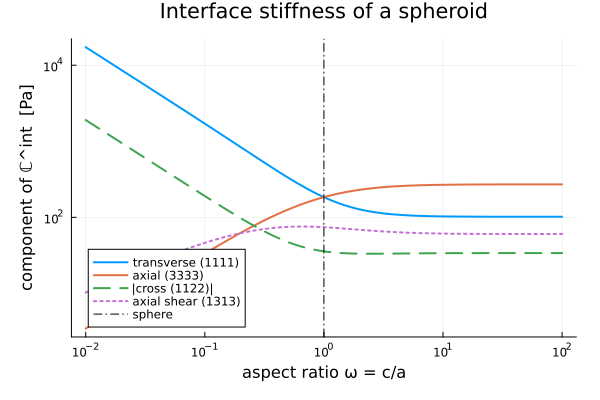
§2 The three limiting cases of the paper
The closed form has a removable singularity at
println("Spherical limit X = 1, closed form:")
R = 1.0
A = canonical_components(surface_stiffness(Ellipsoid(R), κs, μs))
@printf "  C_1111 = %.6f   vs  8(κs+μs)/(5R) = %.6f\n" A[1, 1, 1, 1] 8 * (κs + μs) / (5R)
@printf "  C_1122 = %.6f   vs  2(3κs-2μs)/(5R) = %.6f\n" A[1, 1, 2, 2] 2 * (3κs - 2μs) / (5R)
@printf "  C_1313 = %.6f   vs  (κs+6μs)/(5R) = %.6f\n" A[1, 3, 1, 3] (κs + 6μs) / (5R)

println("\nAsymptotic oblate limit X → 0 (platelet):")
c = 1.0e-6
B = canonical_components(surface_stiffness(Ellipsoid(1.0, 1.0, c), κs, μs))
@printf "  c·C_1111 = %.6f   vs  3(κs+μs)/2 = %.6f\n" c * B[1, 1, 1, 1] 3 * (κs + μs) / 2
@printf "  c·C_1122 = %.6f   vs  3(κs-μs)/2 = %.6f\n" c * B[1, 1, 2, 2] 3 * (κs - μs) / 2
@printf "  c·C_1212 = %.6f   vs  3μs/2      = %.6f\n" c * B[1, 2, 1, 2] 3μs / 2
@printf "  c·C_3333 = %.3e  (vanishes: a platelet stiffens only in its plane)\n" c * B[3, 3, 3, 3]

println("\nAsymptotic prolate limit X → ∞ (nanofiber):")
D = canonical_components(surface_stiffness(Ellipsoid(1.0e6, 1.0, 1.0), κs, μs))
@printf "  axial   C = %.6f   vs  3π(κs+μs)/(4a) = %.6f\n" D[1, 1, 1, 1] 3π * (κs + μs) / (4a)
@printf "  C_1111/C_1122 = %.6f   vs  3 (compared with atomistics in the paper)\n" D[2, 2, 2, 2] / D[2, 2, 3, 3]
Spherical limit X = 1, closed form:
C_1111 = 184.480000 vs 8(κs+μs)/(5R) = 184.480000
C_1122 = 35.760000 vs 2(3κs-2μs)/(5R) = 35.760000
C_1313 = 74.360000 vs (κs+6μs)/(5R) = 74.360000
Asymptotic oblate limit X → 0 (platelet):
c·C_1111 = 172.950000 vs 3(κs+μs)/2 = 172.950000
c·C_1122 = 19.050000 vs 3(κs-μs)/2 = 19.050000
c·C_1212 = 76.950000 vs 3μs/2 = 76.950000
c·C_3333 = 3.459e-10 (vanishes: a platelet stiffens only in its plane)
Asymptotic prolate limit X → ∞ (nanofiber):
axial C = 271.669225 vs 3π(κs+μs)/(4a) = 271.669225
C_1111/C_1122 = 3.000000 vs 3 (compared with atomistics in the paper)§3 The size effect
k_m, μ_m = 30.0, 20.0                       ## a polymer-like matrix, GPa
C_m = TensISO{3}(3k_m, 2μ_m)
C_i = TensISO{3}(3 * 120.0, 2 * 80.0)       ## a stiff filler
f = 0.15

function mt_with_interface(radius; with_interface = true)
    sph = Ellipsoid(radius)
    C_eq = with_interface ? equivalent_particle(C_i, sph, κs * 1.0e-9, μs * 1.0e-9) : C_i
    rve = RVE()
    add_phase!(rve, :M, Ellipsoid(1.0), Dict(:C => C_m); fraction = :rest)
    add_phase!(rve, :nano, sph, Dict(:C => C_eq); fraction = f)
    return canonical_components(homogenize(rve, MoriTanaka(), :C))[1, 2, 1, 2]
end

radii = 10.0 .^ range(-9, -6; length = 60)       ## 1 nm to 1 μm
μ_nano = [mt_with_interface(r) for r in radii]
μ_bulk = mt_with_interface(1.0; with_interface = false)

@printf "\nMori-Tanaka with the equivalent particle, f = %.2f:\n" f
for r in (1.0e-9, 5.0e-9, 2.0e-8, 1.0e-7)
    @printf "  radius %6.1f nm :  μ_eff = %.4f GPa   (+%.1f %% vs no interface)\n" r * 1.0e9 mt_with_interface(r) 100 * (mt_with_interface(r) / μ_bulk - 1)
end

p2 = plot(
    radii .* 1.0e9, μ_nano; xscale = :log10,
    xlabel = "particle radius [nm]", ylabel = "μ^hom  [GPa]",
    title = "Size effect through the equivalent particle",
    label = "with interface", lw = 2, legend = :topright
)
hline!(p2, [μ_bulk]; ls = :dash, label = "no interface")
p2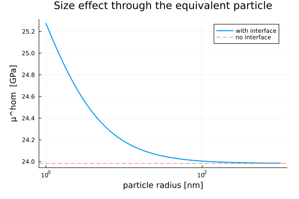
§4 Shape at fixed volume fraction
Platelets and fibers do not stiffen the same way: the oblate limit concentrates the interface effect in the plane of the particle, the prolate one spreads it over every component.
Xs2 = 10.0 .^ range(-1.5, 1.5; length = 40)
μ_shape = Float64[]
for X in Xs2
    # Fixed particle volume, varying aspect ratio.
    a0 = (1.0e-8^3 / X)^(1 / 3)
    ell = X < 1 ? Ellipsoid(a0, a0, X * a0) : Ellipsoid(X * a0, a0, a0)
    C_eq = equivalent_particle(C_i, ell, κs * 1.0e-9, μs * 1.0e-9)
    rve = RVE()
    add_phase!(rve, :M, Ellipsoid(1.0), Dict(:C => C_m); fraction = :rest)
    add_phase!(rve, :nano, ell, Dict(:C => C_eq); fraction = f, symmetrize = :iso)
    push!(μ_shape, canonical_components(homogenize(rve, MoriTanaka(), :C))[1, 2, 1, 2])
end

p3 = plot(
    Xs2, μ_shape; xscale = :log10,
    xlabel = "aspect ratio ω = c/a", ylabel = "μ^hom  [GPa]",
    title = "Orientation-averaged, fixed volume and fraction",
    label = "with interface", lw = 2, legend = :bottomright
)
vline!(p3, [1.0]; color = :black, ls = :dashdot, label = "sphere")
p3

p_full = plot(p1, p2, p3; layout = (1, 3), left_margin = 8Plots.mm, bottom_margin = 8Plots.mm,
    size = (1500, 520), titlefontsize = 9)
p_full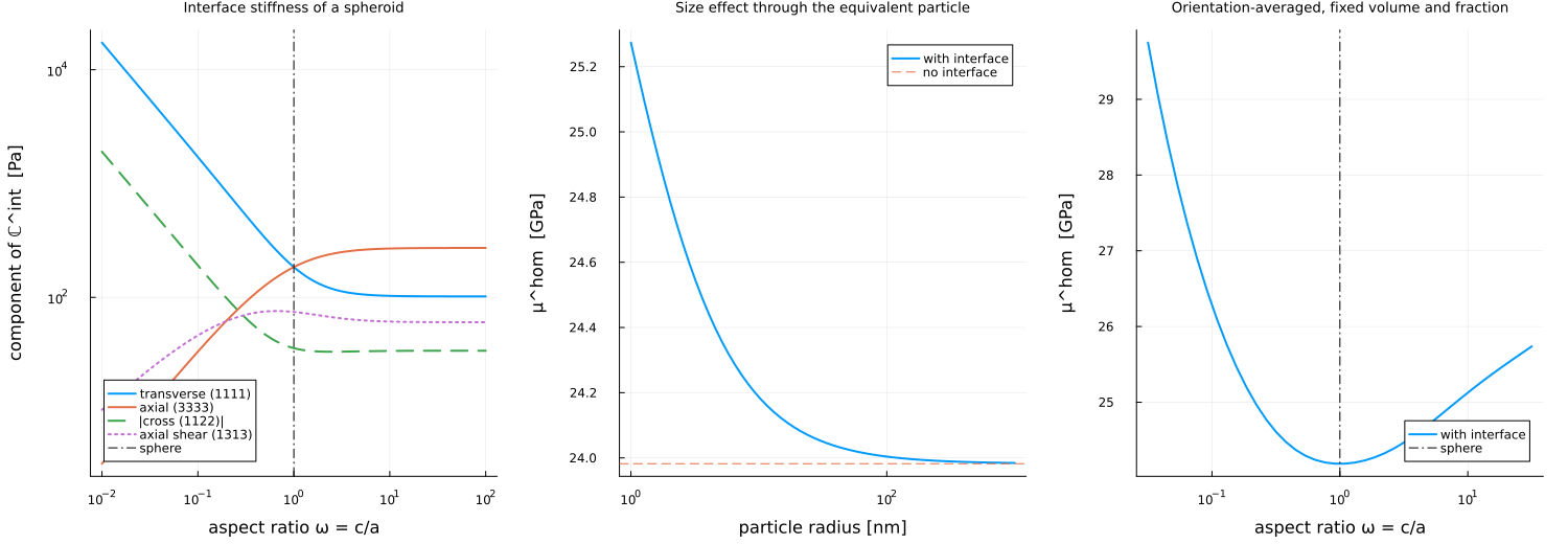
The last figure sets the three preceding panels side by side: the interface stiffness against the aspect ratio, the size effect on a sphere, and the shape effect at fixed particle volume.
Where to go next
This closes the problems of a single heterogeneity. The schemes that turn their solutions into effective properties come next, from Porous materials: the self-consistent trap and every scheme. A planar interface carries the same surface elasticity without any particle around it: Imperfect interfaces in a laminate, and the size effect, in the same group, returns to the size effect met here. The syntax of equivalent_particle is recalled in Particle assemblies and N-body schemes of the manual.
This page was generated using Literate.jl.