Mori–Tanaka

Before this page

Dilute estimates, whose auxiliary problem is kept here with a different remote field, and Homogenization schemes for the identity    .

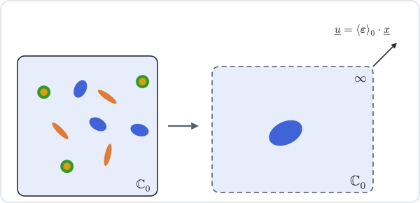
The dilute estimate violates the strain average because each inclusion is loaded by the macroscopic strain while the matrix around it is not. The scheme of Mori and Tanaka (1973), in the form given by Benveniste (1987), repairs this with one change: each inclusion is still alone in the matrix, but the strain it sees at infinity is the mean strain of the matrix,  .

1. The estimate

The dilute solution then gives   , and the strain average fixes the mean matrix strain:

The concentration tensors and the estimate follow,

The inverse stands on the right of : it maps the macroscopic strain to the mean strain of the matrix, on which the contributions act. With     and   , the bracket is    , so that

This second form is the one to keep in mind for the next page: it differs from the Maxwell estimate only in the tensor that multiplies each contribution in the bracket.

2. Cracks

A crack family adds the two limits of §2 of the overview:     to the bracket and       to . With cracks alone, writing    ,

which is the non-interaction approximation of the dual dilute estimate: for cracks, Mori–Tanaka and DiluteDual coincide. The crack term in the bracket is not optional: an additive crack term alone would make the stiffness vanish at a moderate density.

3. Concentration tensors

Unlike most schemes, Mori–Tanaka starts from its concentration tensors, and in the terms of the overview the remote field is the mean strain of the matrix,

the crack families included. The matrix taking the rest of the strain average,       , the definition of returns  : the scheme is consistent with its own premise.

4. Properties

For a two-phase isotropic composite with spherical inclusions and well-ordered phases, the estimate coincides with a bound of Hashin and Shtrikman (1963): the upper bound when the matrix is the stiffer phase, the lower one when it is the softer.

With several inclusion shapes the estimate is not, in general, major-symmetric. Ponte Castañeda and Willis (1995) trace this to the morphology the scheme implicitly assumes, which the page on their estimate makes explicit. The package returns the estimate as computed: an asymmetric Mori–Tanaka tensor is the scheme's answer, not a numerical artifact.

The scheme reads one phase as the matrix, and the estimate depends on that choice (Who is the matrix?). In conduction it is the same formula with in place of .

Where to go next

Mori–Tanaka describes what surrounds an inclusion only through the mean strain of the matrix. The next two pages add a second shape, which describes how the inclusions are distributed: Maxwell through the far field of a cluster, then Ponte Castañeda–Willis through an energy principle and the two-point statistics, which recovers Mori–Tanaka as a particular choice of distribution. The estimate is computed and compared with the bounds in the tutorial Bounds and classical schemes.