Quickstart: a structure with a nonlinear law

The whole path from a law to a structural computation, in one script: a thick tube of an elastoplastic steel, inflated by an internal pressure until it almost collapses. The law is a J2Plasticity of MaterialLaws; the mesh, the assembly and the boundary conditions are Ferrite's; MeanFieldHomogenization provides the element, the global Newton iteration and the output. Step by step explains every line.

using MeanFieldHomogenization, Ferrite

a, b, σ₀ = 1.0, 2.0, 250.0                         # radii (m), yield stress (MPa)
law = J2Plasticity(; E = 200e3, ν = 0.3, σ₀)        # perfectly plastic steel

# A quarter of the tube in plane strain: a square bent into (r, θ), quadratic elements.
grid = generate_grid(QuadraticQuadrilateral, (8, 6), Vec(0.0, 0.0), Vec(1.0, 1.0))
transform_coordinates!(grid, x -> (r = a + (b - a) * x[1]; θ = π / 2 * x[2]; Vec(r * cos(θ), r * sin(θ))))
ip, ip_geo = Lagrange{RefQuadrilateral, 2}()^2, Lagrange{RefQuadrilateral, 2}()
cv = CellValues(QuadratureRule{RefQuadrilateral}(3), ip, ip_geo)
dh = close!(add!(DofHandler(grid), :u, ip))
ch = ConstraintHandler(dh)                          # the two planes of symmetry
add!(ch, Dirichlet(:u, getfacetset(grid, "bottom"), (x, t) -> 0.0, [2]))
add!(ch, Dirichlet(:u, getfacetset(grid, "top"), (x, t) -> 0.0, [1]))
close!(ch)

# The nodal forces of a unit pressure on the inner surface.
fv = FacetValues(FacetQuadratureRule{RefQuadrilateral}(3), ip, ip_geo)
f_unit = zeros(ndofs(dh))
for facet in FacetIterator(dh, getfacetset(grid, "left"))
    reinit!(fv, facet)
    fe = zeros(ndofs_per_cell(dh))
    for q in 1:getnquadpoints(fv), i in eachindex(fe)
        fe[i] -= (shape_value(fv, q, i) ⋅ getnormal(fv, q)) * getdetJdV(fv, q)
    end
    assemble!(f_unit, celldofs(facet), fe)
end

# The computation: pressure raised to 97 % of the limit pressure in 25 steps.
p_lim = 2σ₀ / sqrt(3) * log(b / a)
pressure(t) = 0.97 * p_lim * t
states = QuadratureStates(law, getncells(grid), getnquadpoints(cv))
system!, prescribe! = material_system(dh, ch, cv, law, PlaneStrain(), states;
    external_forces! = (r, t) -> (r .-= pressure(t) .* f_unit))
u = zeros(ndofs(dh))
times = range(0, 1; length = 26)
u_inner = [0.0]                                     # radial displacement of the bore
quasistatic!(system!, prescribe!, u, states, times;
    on_step = (i, t, u, st) -> push!(u_inner, evaluate_at_grid_nodes(dh, u, :u)[1][1]))
write_material_vtk(joinpath(mktempdir(), "tube"), dh, u, law, states)   # for ParaView

The response, against the limit pressure of the tube:

using Plots
plot(u_inner * 1e3, pressure.(times); lw = 2, label = "finite elements, J2Plasticity",
    xlabel = "radial displacement of the bore (mm)", ylabel = "internal pressure (MPa)", legend = :bottomright)
hline!([p_lim]; ls = :dash, label = "limit pressure (2σ₀/√3) ln(b/a)")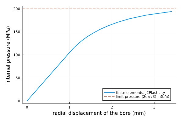

The pressure first rises linearly (elastic tube), then bends as the plastic zone spreads from the bore outward, and flattens under the limit pressure.

Where the limit pressure comes from

At collapse the plastic flow dominates and is incompressible, so that in plane strain the axial stress is the mean of the two others, and the von Mises criterion reads   . With the radial equilibrium   , a tube plastic throughout integrates from   to   :  . No pressure beyond it can be carried by a perfectly plastic material.

Every step converged in a handful of global Newton iterations, the mark of a consistent tangent. The VTK file holds the displacement and, cell by cell, the stress (σ11, …), the strain (ε11, …) and the internal variables of the law (p, εᵖ11, …), to open in ParaView.