Getting started

This page takes a first calculation from the installation of the package to an effective stiffness: a matrix carrying spherical inclusions is described, one homogenization scheme is applied to it, and the effective moduli are read back. No familiarity with mean-field homogenization is assumed beyond linear elasticity; each quantity is defined in the chapter Theory, to which the text refers where the quantity is first needed.

Installation

MeanFieldHomogenization is registered in Julia's General registry and is installed with the package manager, either from the Pkg mode of the REPL (entered by typing ])

pkg> add MeanFieldHomogenization

or, equivalently, through the Pkg API:

julia> import Pkg; Pkg.add("MeanFieldHomogenization")

No additional registry is required: the dependencies (TensND.jl, OrdinaryDiffEqTsit5.jl, Elliptic.jl, QuadGK.jl, Polynomials.jl, Tensors.jl, …) come from General as well, and the type-generic elliptic integrals are bundled as the MeanFieldHomogenization.Elliptic submodule.

Optional package extensions

Nothing below is needed for the core. Each extension loads by itself when its trigger packages are imported, and the feature it unlocks is the only thing that is unavailable without it.

Load	Unlocks
DECUHR, Integrals	the adaptive-cubature backend method = :decuhr for arbitrary anisotropy; the bundled method = :nestedquadgk covers the same cases
NonlinearSolve	any SciML algorithm for the self-consistent fixed points (Iterative solvers)
SymPyPythonCall	symbolic closed forms of the elliptic integrals
Ferrite, FerriteGmsh, Gmsh	the reference finite-element backend for FE inclusions
Gridap, GridapGmsh	the second FE backend for the same morphologies
Ferrite (alone)	the material interface of the finite-element coupling — a microstructure as a Gauss-point law
Lux, Optimisers, Zygote	training a neural surrogate; evaluating a shipped model needs none of them

A first estimate

A matrix of bulk modulus   GPa and shear modulus   GPa carries spherical inclusions twice as stiff, at a volume fraction  . The microstructure is described by a representative volume element (RVE), a container to which each phase is added with its geometry, its properties and its amount:

using MeanFieldHomogenization

rve = RVE()
add_phase!(rve, :M, Ellipsoid(1.0), Dict(:C => iso_stiffness(30.0, 10.0)); fraction = :rest)
add_phase!(rve, :I, Ellipsoid(1.0), Dict(:C => iso_stiffness(60.0, 20.0)); fraction = 0.2)
rve

RVE{Float64} with 2 phase(s)
  phase :M   f = 0.8  (rest)
  phase :I   f = 0.2
  closure : ComplementFraction(:warn)
  distribution_shape : none declared (Maxwell / PCW will ask for one)

Ellipsoid(1.0) is a sphere, iso_stiffness(k, mu) the isotropic stiffness tensor of bulk modulus k and shear modulus mu, and fraction = :rest gives the matrix whatever volume the other phases leave. The RVE says nothing about which phase plays the role of a matrix: that is decided by the scheme (Who is the matrix?).

The Mori–Tanaka scheme takes the matrix as the reference medium, of stiffness , and loads each inclusion with the average strain of the matrix. With the dilute concentration tensor of the inclusion phase ,

where is the Hill polarization tensor of the inclusion shape in the reference medium (Hill polarization tensors), the estimate of the effective stiffness reads

with the volume fraction of the matrix. homogenize evaluates it for the property :C of the RVE, and k_mu (from TensND) reads back the bulk and shear moduli of the isotropic result:

C_hom = homogenize(rve, MoriTanaka(), :C)
k_mu(C_hom)

(33.86138613861386, 11.460674157303371)

Changing the estimate means changing the scheme argument only: Dilute(), SelfConsistent(), DifferentialScheme() and the bounds Voigt() and Reuss() are called the same way, and what each assumes is the subject of Homogenization schemes.

Where to go next

The documentation can be entered from three directions, depending on what the reader already knows.

• A reader new to mean-field homogenization is best served by the chapter Theory read in its stated order, from The Eshelby problem to Homogenization schemes, before the tutorial A first homogenization, which compares two schemes on the RVE above.

• A reader who knows what is to be computed can go to Schemes and RVEs, then to the page of the Manual that matches the morphology at hand.

• A user of Echoes will find the correspondence between the two libraries in From Echoes to MeanFieldHomogenization.

An alternative to scripting: MFH Studio

MeanFieldHomogenization is a library driven from Julia, as on this page. The same models can also be built with forms, in the browser, with MFH Studio: describe each phase, choose the schemes, run, and read the Julia script it writes as you go, which runs on its own. It ships with the package:

julia> using MeanFieldHomogenization; mfhstudio()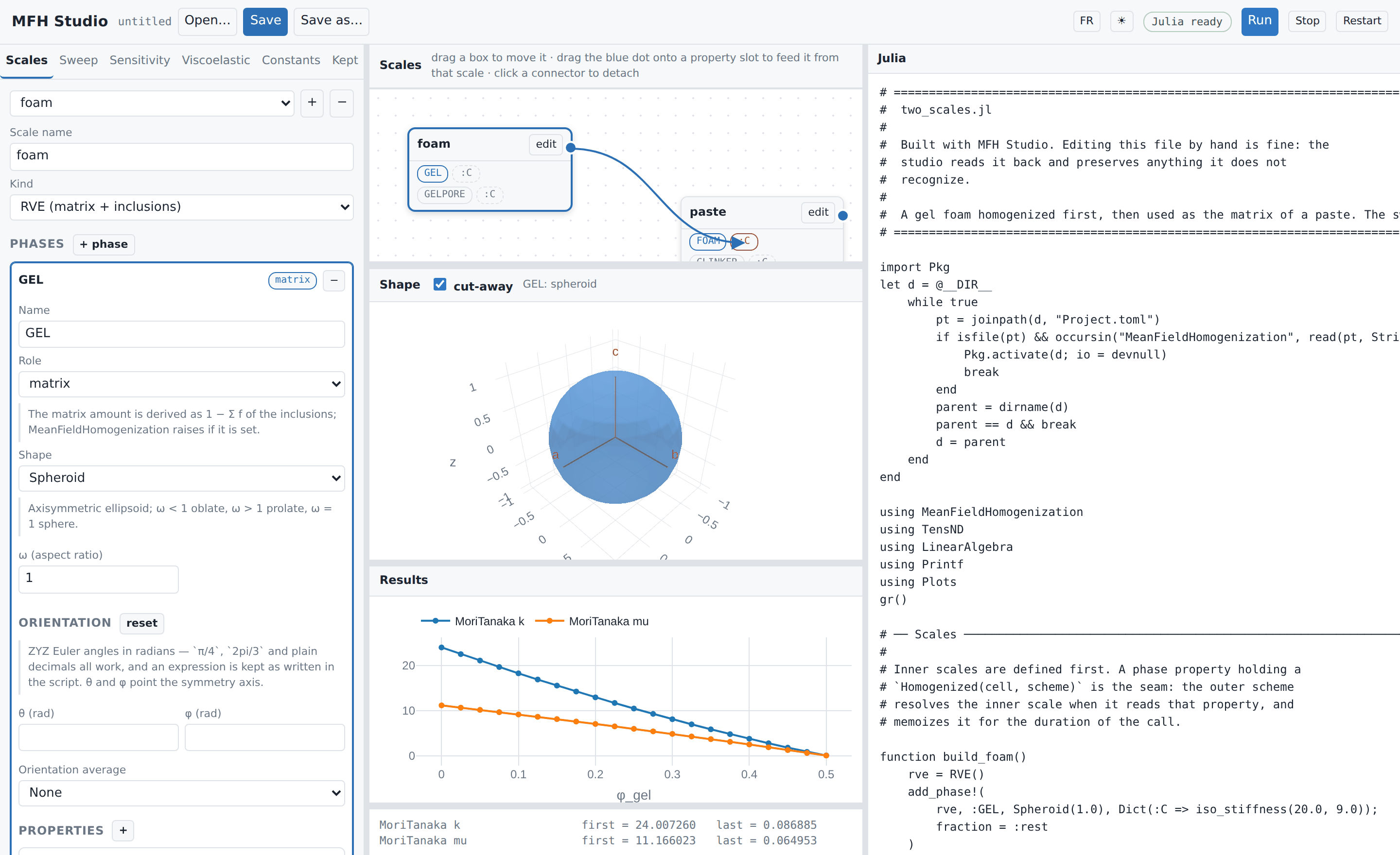

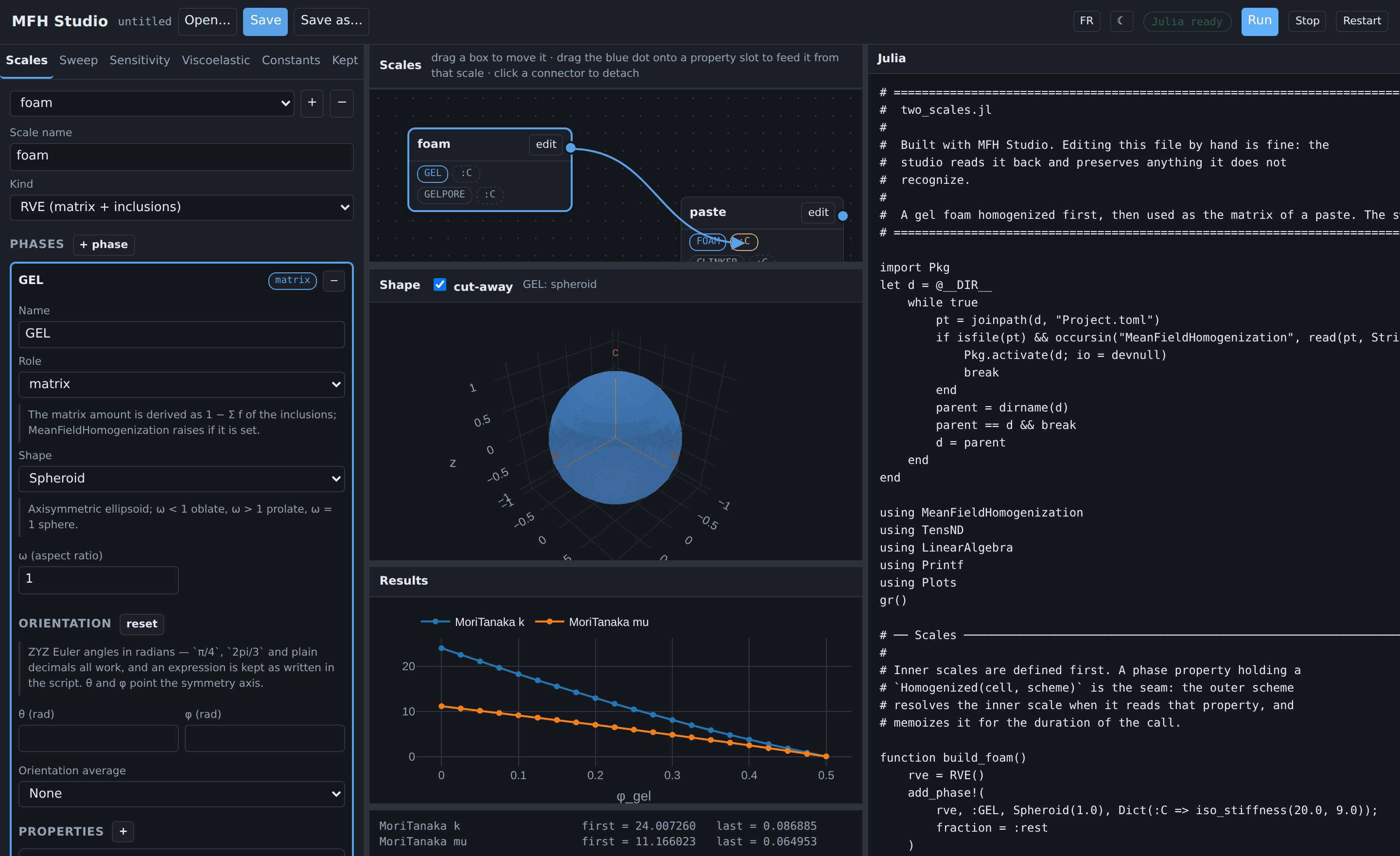
Ten worked examples open with every form filled in (Start here).

Citing MeanFieldHomogenization

When MeanFieldHomogenization is used in published work, it is to be cited as follows; CITATION.cff in the repository root carries the same metadata in a machine-readable form.

@software{meanfieldhomogenization_jl,
  author = {Barthélémy, Jean-François},
  title  = {MeanFieldHomogenization.jl: Mean-field homogenization of heterogeneous materials},
  doi    = {10.5281/zenodo.21884243},
  url    = {https://doi.org/10.5281/zenodo.21884243},
}