n-layer sphere: volume-averaged concentration tensors

The whole page as one script

Every block of this page, in order, is scripts/30_average_nlayers.jl. From a clone of the repository, julia --project=docs -e 'using Pkg; Pkg.instantiate()' once, then julia scripts/30_average_nlayers.jl, runs it end to end.

Before this page

The tutorial Hill polarization tensors in practice, whose dilute estimate built from one concentration tensor is extended here to an inclusion of several layers, and the theory page Layered sphere — bulk + shear recurrences and imperfect interfaces, where the recurrence evaluated below is derived.

Volume-averaged strain and stress concentration tensors of an isotropic n-layer composite sphere. Uses random per-layer moduli and a random reference matrix, and adds a per-layer bar chart of the bulk and shear concentration factors .

The MeanFieldHomogenization.jl API used here:

LayeredSphere(radii, moduli) — geometry + per-layer stiffness;
gradient_gradient_concentration(sphere, C₀; layer=k) — per-layer iso ;
property_contribution(sphere, C₀) — size-independent ;
layer_volume_fraction(sphere, k) — .

The whole-inclusion average

is reconstructed and cross-checked against the dilute-scheme identity .

julia

using MeanFieldHomogenization
using TensND
using Random
using Printf
using LinearAlgebra
using Plots
gr()  # headless backend; GKSwstype is set to "100" before Literate runs

default(; left_margin = 5Plots.mm, bottom_margin = 5Plots.mm)

Helpers

for direct TensISO{3} construction.

julia

function _stiff_Enu(E::Real, ν::Real)
    K = E / (3 * (1 - 2ν))
    μ = E / (2 * (1 + ν))
    return TensISO{3}(3K, 2μ)
end

_iso_Kμ(C::TensISO{4, 3}) = (TensND.get_data(C)[1] / 3, TensND.get_data(C)[2] / 2)

_iso_Kμ (generic function with 1 method)

Convert layer fractions (positive, sum = 1 expected) to ascending radii given a target outer radius R. Layer k occupies r_{k-1}..r_k with .

julia

function _radii_from_fractions(f::AbstractVector{<:Real}, R::Real)
    @assert all(>(0), f) "layer fractions must be > 0"
    f_norm = f ./ sum(f)
    cum = zero(R)
    radii = similar(f_norm, typeof(R))
    for k in eachindex(f_norm)
        cum += f_norm[k] * R^3
        radii[k] = cbrt(cum)
    end
    return Tuple(radii)
end

_radii_from_fractions (generic function with 1 method)

Setup — random n-layer sphere + random reference

The seed is fixed so this page (and the standalone script) render identical numbers every time.

julia

Random.seed!(20260426)

const n = 10
const R = 5.0

5.0

Random layer fractions (Dirichlet-ish: independent uniforms re-normalized).

julia

const fractions = rand(n) .+ 0.05
const fractions_n = fractions ./ sum(fractions)

10-element Vector{Float64}:
 0.04188744832859412
 0.1502885935502196
 0.12653284462817221
 0.10578112193381599
 0.08816122027900777
 0.11898276511810135
 0.01074705671259343
 0.10129186760080625
 0.11364956667923229
 0.14267751516945706

Random per-layer moduli (E, ν).

julia

const E_rand = 1.0 .+ 9.0 .* rand(n)
const ν_rand = 0.05 .+ 0.4 .* rand(n)
const C_layers = ntuple(k -> _stiff_Enu(E_rand[k], ν_rand[k]), n)

((9.164315611938743) 𝕁 + (5.565801032055056) 𝕂, (15.428685642373036) 𝕁 + (4.794304763087126) 𝕂, (6.7127163236238605) 𝕁 + (3.404367869000236) 𝕂, (19.821121489046263) 𝕁 + (5.294917734460735) 𝕂, (3.6597110689076744) 𝕁 + (1.4926496350361154) 𝕂, (5.207126418398294) 𝕁 + (4.252027983390384) 𝕂, (20.096585612688358) 𝕁 + (2.5294463492480213) 𝕂, (6.427895662994883) 𝕁 + (5.282731686913854) 𝕂, (13.253897399340591) 𝕁 + (7.2117468011312384) 𝕂, (12.879540953436193) 𝕁 + (3.8589800941473342) 𝕂)

Random reference (matrix) modulus.

julia

const C_ref = _stiff_Enu(1.0 + 9.0 * rand(), 0.05 + 0.4 * rand())

const radii = _radii_from_fractions(fractions_n, R)
const sphere = LayeredSphere(radii, C_layers)

LayeredSphere{Float64} (10 layer(s), radii = (1.7364594232161372, 2.8853804557734475, 3.4153461663808145, 3.757732218944052, 4.001695189606067, 4.290011957985785, 4.314206327331856, 4.529990867323564, 4.749903017097512, 5.0))

Summary

julia

println("Random n-layer sphere — n = $n, R = $R")
println("─"^78)
println("Per-layer (E, ν) :")
for k in 1:n
    @printf "  k=%2d  E = %6.3f  ν = %5.3f\n" k E_rand[k] ν_rand[k]
end
println()

K_ref, μ_ref = _iso_Kμ(C_ref)
@printf "Reference matrix : K_ref = %.5f, μ_ref = %.5f\n" K_ref μ_ref
println()

println("Geometry :")
@printf "  outer radius          : %.5f\n" radii[end]
@printf "  Σ layer_fraction      : %.10f  (should be 1)\n" sum(
    layer_volume_fraction(sphere, k) for k in 1:n
)
println("  layer_radius          : ", join(map(r -> @sprintf("%.4f", r), radii), ", "))
println(
    "  layer_volume_fraction : ", join(
        map(k -> @sprintf("%.5f", layer_volume_fraction(sphere, k)), 1:n), ", "
    )
)
println()

Random n-layer sphere — n = 10, R = 5.0
──────────────────────────────────────────────────────────────────────────────
Per-layer (E, ν) :
  k= 1  E =  6.404  ν = 0.151
  k= 2  E =  6.224  ν = 0.298
  k= 3  E =  4.074  ν = 0.197
  k= 4  E =  7.007  ν = 0.323
  k= 5  E =  1.860  ν = 0.246
  k= 6  E =  4.529  ν = 0.065
  k= 7  E =  3.570  ν = 0.411
  k= 8  E =  5.616  ν = 0.063
  k= 9  E =  8.504  ν = 0.179
  k=10  E =  5.034  ν = 0.305

Reference matrix : K_ref = 4.14995, μ_ref = 3.15322

Geometry :
  outer radius          : 5.00000
  Σ layer_fraction      : 1.0000000000  (should be 1)
  layer_radius          : 1.7365, 2.8854, 3.4153, 3.7577, 4.0017, 4.2900, 4.3142, 4.5300, 4.7499, 5.0000
  layer_volume_fraction : 0.04189, 0.15029, 0.12653, 0.10578, 0.08816, 0.11898, 0.01075, 0.10129, 0.11365, 0.14268

Per-layer concentration tensors (iso 4-tensor)

julia

A_per_layer = ntuple(k -> gradient_gradient_concentration(sphere, C_ref; layer = k), n)
αβ = ntuple(k -> TensND.get_data(A_per_layer[k]), n)
α_k = [αβ[k][1] for k in 1:n]   # bulk concentration
β_k = [αβ[k][2] for k in 1:n]   # shear concentration

println("Per-layer concentration factors :")
@printf "  %-4s  %-12s  %-12s\n" "k" "α_k (bulk)" "β_k (shear)"
for k in 1:n
    @printf "  %2d    %+10.6f    %+10.6f\n" k α_k[k] β_k[k]
end
println()

Per-layer concentration factors :
  k     α_k (bulk)    β_k (shear)
   1     +1.045775     +1.018958
   2     +0.783911     +1.065978
   3     +1.277488     +1.254331
   4     +0.694112     +0.992759
   5     +2.107171     +2.108761
   6     +1.478530     +1.169814
   7     +0.641448     +1.488498
   8     +1.335576     +1.059136
   9     +0.988815     +0.943263
  10     +0.944056     +1.253558

Whole-inclusion average (perfect interfaces).

julia

A_whole_α = sum(layer_volume_fraction(sphere, k) * α_k[k] for k in 1:n)
A_whole_β = sum(layer_volume_fraction(sphere, k) * β_k[k] for k in 1:n)
@printf "Whole-inclusion average :  α = %+12.8f   β = %+12.8f\n" A_whole_α A_whole_β

Whole-inclusion average :  α =  +1.14762696   β =  +1.20104848

Cross-check: property_contribution satisfies .

julia

N_tensor = property_contribution(sphere, C_ref)
N_α, N_β = TensND.get_data(N_tensor)
N_α_check = sum(
    layer_volume_fraction(sphere, k) *
        (TensND.get_data(C_layers[k])[1] - TensND.get_data(C_ref)[1]) *
        α_k[k] for k in 1:n
)
N_β_check = sum(
    layer_volume_fraction(sphere, k) *
        (TensND.get_data(C_layers[k])[2] - TensND.get_data(C_ref)[2]) *
        β_k[k] for k in 1:n
)
@printf "property_contribution :  N_α = %+12.6f  (rec. %+12.6f, diff=%.2e)\n" N_α N_α_check abs(N_α - N_α_check)
@printf "                         N_β = %+12.6f  (rec. %+12.6f, diff=%.2e)\n" N_β N_β_check abs(N_β - N_β_check)
println()

property_contribution :  N_α =    -3.699935  (rec.    -3.699935, diff=0.00e+00)
                         N_β =    -2.532505  (rec.    -2.532505, diff=0.00e+00)

Reset reference to last-layer modulus (mirror Python l. 59-60)

julia

println("Resetting reference to C_layers[end] :")
C_ref2 = C_layers[end]
A_layer_last = gradient_gradient_concentration(sphere, C_ref2; layer = n)
α_last, β_last = TensND.get_data(A_layer_last)
@printf "  layer_eE(n) with C_ref = C_layers[n] :  α = %+10.6f  β = %+10.6f\n" α_last β_last
println("  (when reference = layer modulus, the layer is invisible to itself.)")
println()

Resetting reference to C_layers[end] :
  layer_eE(n) with C_ref = C_layers[n] :  α =  +1.000000  β =  +1.000000
  (when reference = layer modulus, the layer is invisible to itself.)

Graphical output

Per-layer bulk/shear concentration factors and volume fractions, bar-charted side by side.

julia

p1 = bar(
    1:n, α_k;
    xlabel = "layer k", ylabel = "α_k (bulk)",
    title = "Bulk concentration per layer",
    legend = false, color = :steelblue
)
hline!(
    p1, [A_whole_α]; lw = 2, color = :red, linestyle = :dash,
    label = "<α> = $(round(A_whole_α; digits = 4))"
)
p1 = plot!(p1; legend = :topright)

p2 = bar(
    1:n, β_k;
    xlabel = "layer k", ylabel = "β_k (shear)",
    title = "Shear concentration per layer",
    legend = false, color = :darkorange
)
hline!(
    p2, [A_whole_β]; lw = 2, color = :red, linestyle = :dash,
    label = "<β> = $(round(A_whole_β; digits = 4))"
)
p2 = plot!(p2; legend = :topright)

p3 = bar(
    1:n, [layer_volume_fraction(sphere, k) for k in 1:n];
    xlabel = "layer k", ylabel = "f_k",
    title = "Layer volume fractions",
    legend = false, color = :seagreen
)

p_full = plot(
    p1, p2, p3; layout = (1, 3), left_margin = 8Plots.mm, bottom_margin = 8Plots.mm,
    size = (1500, 520), titlefontsize = 9,
    plot_title = "n-layer sphere ($n layers, R=$R) — average concentrations"
)
p_full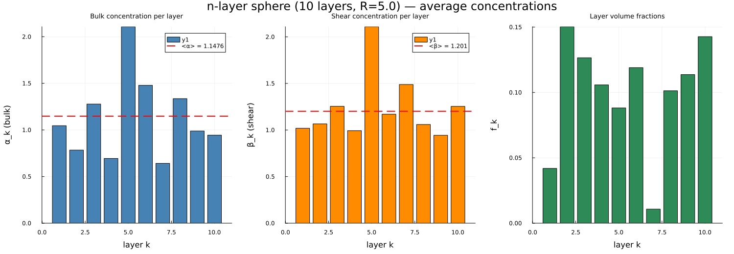

Each bar is the concentration factor of one layer, and the dashed line is their volume-weighted average, which is the factor the inclusion as a whole presents to a scheme.

Standalone run also saves the figure to scripts/figures/:

Where to go next

A layer average says nothing about where, inside a layer, the strain concentrates. n-layer sphere: pointwise fields evaluates the strain, stress and displacement at a point of the same kind of sphere, with perfect or imperfect interfaces, and checks that the field averages back to the layer factors computed here. The constructors and the interface laws of LayeredSphere are documented in Layered inclusions of the manual.

This page was generated using Literate.jl.

n-layer sphere: volume-averaged concentration tensors ​

Helpers ​

Setup — random n-layer sphere + random reference ​

Summary ​

Per-layer concentration tensors (iso 4-tensor) ​

Reset reference to last-layer modulus (mirror Python l. 59-60) ​

Graphical output ​

Where to go next ​

n-layer sphere: volume-averaged concentration tensors

Helpers

Setup — random n-layer sphere + random reference

Summary

Per-layer concentration tensors (iso 4-tensor)

Reset reference to last-layer modulus (mirror Python l. 59-60)

Graphical output

Where to go next