The equivalent inclusion method

Before this page

Two-inclusion interaction tensors, where and the Green operator are defined, and The cluster model, to which §3 relates the method.

The equivalent inclusion method of Brisard et al. (2014) is a Galerkin discretization of the weak form of the Lippmann-Schwinger equation, with the polarization taken piecewise polynomial over the inclusions. Unlike every other scheme of the package it also delivers a rigorous bound on the apparent stiffness.

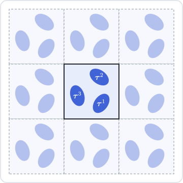
Where Moschovidis and Mura (1975) discretized the strong form by Taylor expansion and collocation, the variational form discretizes the weak one — and inherits the extremum property of the Hashin-Shtrikman principle.

Notation as in the Nomenclature; the interaction tensor and the Green operator are defined on the interaction page.

1. Variational form

The modified Lippmann-Schwinger equation of (Brisard et al., 2013), posed on an ellipsoidal statistical volume element embedded in an infinite medium of the matrix stiffness, has the weak form: find   such that   for every  , with

The last term of comes from Eshelby's theorem applied to the SVE itself — legitimate because is an ellipsoid — and is its Hill tensor. It is what implements the mixed boundary conditions: a uniform strain at infinity plus a uniform surface traction chosen so that the loading parameter coincides with the macroscopic strain.

2. Galerkin discretization

Take the polarization piecewise polynomial of degree over each inclusion,

with the indicator function of . This is their discrete problem. At   — one constant polarization per inclusion — dividing by gives

Local fields come out for free:     and    . Solving the system for a unit macroscopic strain, the polarization of each particle is a fourth-order tensor applied to , and so is its mean strain: these are the concentration tensors that concentration_tensors returns, one per particle, in the form of the overview, the matrix closing both averages.

Transcribed verbatim

The package shares the sign convention of Brisard et al. (2023) (see the convention note), so the system above is transcribed with nothing flipped: the self term is , which is , and every block carries a plus. It is the cluster model page that has a flip to declare.

3. Relation to the cluster model

Brisard et al. (2014) observes that at    the influence pseudotensors coincide with the interaction tensors of Berveiller et al. (1987) and Molinari and El Mouden (1996). The two schemes of this package accordingly share interaction_tensor, and differ only in how the far field is closed:

	far-field term	boundary treatment
EquivalentInclusion	, Hill tensor of the SVE	MixedBC — no periodization
ClusterModel	, Hill tensor of the inclusion shape	PeriodicBox — cluster cutoff

Under a PeriodicBox the first reduces to the second, and the two agree to machine precision — the acceptance gate of the implementation.

Two further exact degeneracies:

• a single spherical particle concentric in a spherical SVE gives  , the self block becomes     , and the scheme is Mori-Tanaka — at every volume fraction, not only in the dilute limit;

• as   both collapse onto Dilute.

4. Bounds

Introducing    , the exact solution satisfies

and the discrete one the same identity with . Since is minimum (resp. maximum) at when   (resp. ) for every :

an upper bound, and a lower one in the opposite case. Two consequences: the estimate improves monotonically as grows (the trial space only gets larger), and mixed contrasts give no bound at all. eim_bound_type reports which case holds.

Taking the polarization constant and equal across all inclusions instead recovers the classical bounds of Hashin and Shtrikman (1962); letting it vary from one inclusion to the next is what sharpens them.

5. Reference results

Brisard et al. (2014), Table 1 — plane strain,   circular pores of radius in a circular SVE of radius  , porosity  ,  , 1000 realizations:

order	bound on	dofs
0		480
1		1440
2		2880
3		4800

with a finite-element reference of   and a Hashin-Shtrikman upper bound of   — the order-zero estimate already improves on the latter by 11 %. Their Table 2, in 3D with polydisperse spherical pores (  of radii , , ,  ,   ) gives   at  . scripts/93 reproduces the   row of Table 1.

Only order = 0 is implemented

Orders   require the influence pseudotensors of the paper's Appendix C. These are not tensors — they need their own change-of-basis machinery — and were generated by the authors with a computer algebra system. Requesting a higher order raises an ArgumentError rather than silently returning the order-zero answer.

6. Slender fibers in conduction

Martin et al. (2023) specialize the method to slender cylinders in steady conduction, taking the polarization polynomial in the axial coordinate and constant across the section. Their interaction coefficients reduce, after a multipole step, to nested one-dimensional integrals along the two axes, and their self-influence coefficients are precomputed by finite elements. The :quadrature back-end of interaction_tensor evaluates the same integrals directly; the axial polynomial enrichment is not implemented.

Where to go next

The last page of the chapter, Levin's theorem, draws from the concentration tensors of any of these schemes the response of the composite to free strains and prestresses of its phases. The table of §5 is reproduced in The equivalent inclusion method, against a published table. The construction of a ParticleAssembly is in Particle assemblies and N-body schemes, and the API entries are in API — Particle assemblies.