
n-layer sphere: pointwise fields
The whole page as one script
Every block of this page, in order, is scripts/31_local_nlayers.jl. From a clone of the repository, julia --project=docs -e 'using Pkg; Pkg.instantiate()' once, then julia scripts/31_local_nlayers.jl, runs it end to end.
Before this page
The tutorial n-layer sphere: volume-averaged concentration tensors, whose layer averages the pointwise fields must reproduce, and the section Pointwise fields of the theory page on the layered sphere, where the fields evaluated below are written out.
The strain, stress and displacement at a point inside — and outside — an n-layer composite sphere, under an arbitrary remote loading, with perfect or imperfect interfaces.
Where layer_gradient_average gives one tensor per layer, the pointwise API gives the field itself:
LayeredSphereFields(sphere, C₀)— solve the recurrence once;local_gradient_gradient_concentration(sol, x)—with local_flux_gradient_concentration,local_gradient_flux_concentration,local_flux_flux_concentrationfor a remote stress;local_gradient,local_flux,local_displacement— the fields for one loading;get_layer(sphere, r; side)— which region a radius belongs to, and which limit is meant exactly on an interface.
TensTI{4,T,6}: six Walpole scalars and an axis, not an 81-component array.
using MeanFieldHomogenization
using TensND
using LinearAlgebra
using Printf
using Plots
gr()

default(; left_margin = 5Plots.mm, bottom_margin = 5Plots.mm)
Setup — a stiff core in a compliant ITZ shell
The classic three-phase model of a cement paste: a stiff aggregate, a compliant interfacial transition zone, and the matrix at infinity.
_stiff_Enu(E, ν) = TensISO{3}(3E / (3 * (1 - 2ν)), 2E / (2 * (1 + ν)))

const C₀ = _stiff_Enu(30.0, 0.3)      # matrix
const Cᵢ = _stiff_Enu(100.0, 0.2)     # core (aggregate)
const Cₛ = _stiff_Enu(10.0, 0.35)      # ITZ shell

const R = 1.0                          # core radius
const Rₛ = 1.5                         # shell outer radius

const sphere = LayeredSphere((R, Rₛ), (Cᵢ, Cₛ))
const sol = LayeredSphereFields(sphere, C₀)
LayeredSphereFields{Float64, 2, 3, LayeredSphere{Float64, 2, Tuple{TensND.TensISO{4, 3, Float64, 2}, TensND.TensISO{4, 3, Float64, 2}}, Tuple{PerfectInterface{Float64}, PerfectInterface{Float64}}}, TensND.TensISO{4, 3, Float64, 2}}(LayeredSphere{Float64} (2 layer(s), radii = (1.0, 1.5)), (74.99999999999999) 𝕁 + (23.076923076923077) 𝕂, ((55.555555555555564, 41.66666666666667), (11.111111111111109, 3.7037037037037033)), (24.999999999999996, 11.538461538461538), ((0.44234257061318083, 0.0), (1.6672912276958363, -1.224948657082656), (1.0, 1.027159236390792)), ((0.3545262663706538, -0.003015513398182379, 0.0, 0.0), (2.007401855326695, -0.01249757515102274, 1.0017092294567367, -2.065054227271925), (1.0, 0.0, -1.7279627527107182, 1.0826253802823422)))Radial profiles under a hydrostatic far field
const εᵥ = 1.0
const ε∞_hyd = εᵥ * TensISO{3}(1.0)

"Radial and hoop stress at radius `r` under the remote loading `ε∞`."
function radial_hoop(sol, r, ε∞; side = :outer)
    σ = local_flux(sol, [r, 0.0, 0.0], ε∞; side)
    return σ[1, 1], σ[2, 2]              # e₁ is radial here, e₂ is a hoop axis
end

rs = range(1.0e-6, 4 * Rₛ; length = 600)
σrr_h = [radial_hoop(sol, r, ε∞_hyd)[1] for r in rs]
σθθ_h = [radial_hoop(sol, r, ε∞_hyd)[2] for r in rs]

σ_far = 3 * (30.0 / (3 * (1 - 2 * 0.3))) * εᵥ   # 3K₀ εᵥ

println("Hydrostatic far field, σ∞ᵢᵢ = 3K₀εᵥ = ", round(σ_far; digits = 4))
@printf "  %-9s  %12s  %12s\n" "r" "σ_rr" "σ_θθ"
for r in (0.5R, R, 0.5(R + Rₛ), Rₛ, 2Rₛ)
    σrr, σθθ = radial_hoop(sol, r, ε∞_hyd)
    @printf "  %-9.4f  %+12.6f  %+12.6f\n" r σrr σθθ
end
Hydrostatic far field, σ∞ᵢᵢ = 3K₀εᵥ = 75.0
r σ_rr σ_θθ
0.5000 +73.723762 +73.723762
1.0000 +73.723762 +46.502681
1.2500 +64.867837 +50.930643
1.5000 +60.953378 +82.023311
3.0000 +73.244172 +75.877914Continuity of the radial traction is a property of the solution, not something imposed on the plot — side = :inner and side = :outer are the two limits at an interface radius.
for r in (R, Rₛ)
    Δ = abs(
        radial_hoop(sol, r, ε∞_hyd; side = :outer)[1] -
            radial_hoop(sol, r, ε∞_hyd; side = :inner)[1]
    )
    @printf "  σ_rr continuity at r = %.2f :  Δ = %.3e\n" r Δ
end
σ_rr continuity at r = 1.00 : Δ = 2.842e-14
σ_rr continuity at r = 1.50 : Δ = 2.132e-14Radial profiles under a deviatoric far field
The deviatoric (
const ε∞_uni = Tens(diagm([0.0, 0.0, 1.0]))TensND.TensCanonical{2, 3, Float64, Tensors.SymmetricTensor{2, 3, Float64, 6}}
→ array: 3×3 Tensors.SymmetricTensor{2, 3, Float64, 6}:
0.0 0.0 0.0
0.0 0.0 0.0
0.0 0.0 1.0
→ basis: 3×3 TensND.Id2{3, Float64}:
1.0 ⋅ ⋅
⋅ 1.0 ⋅
⋅ ⋅ 1.0Note the two spellings of a point: a Cartesian vector, as here, or the three separate arguments (r, θ, φ). local_flux(sol, a, b, c, ε∞) is the SPHERICAL form — passing Cartesian components that way silently evaluates somewhere else entirely.
"σ in the meridian plane φ = 0, at colatitude θ, in the canonical basis."
σ_at(sol, r, θ, ε∞; side = :outer) =
    local_flux(sol, [r * sin(θ), 0.0, r * cos(θ)], ε∞; side)

σzz_pole = [σ_at(sol, r, 0.0, ε∞_uni)[3, 3] for r in rs]      # along the load axis
σzz_eq = [σ_at(sol, r, π / 2, ε∞_uni)[3, 3] for r in rs]      # perpendicular to it
600-element Vector{Float64}:
44.2704909435425
44.270101861534485
44.26893477085288
44.26698967149767
44.264266563468865
44.26076544676645
44.25648632139044
44.25142918734084
44.24559404461764
44.23898089322084
⋮
40.43726605917158
40.43697206869866
40.436680289943155
40.436390701985744
40.43610328414512
40.43581801597468
40.43553487725957
40.43525384801346
40.4349749084757A spring interface debonds the core
SpringInterface(kn, kt) takes the interface stiffnesses; the softer the interface, the larger the displacement jump it allows. The traction stays continuous.
const sphere_spring = LayeredSphere(
    (R, Rₛ), (Cᵢ, Cₛ);
    interfaces = (SpringInterface(20.0, 12.0), PerfectInterface{Float64}())
)
const sol_spring = LayeredSphereFields(sphere_spring, C₀)

let n = [1.0, 0.0, 0.0], x = R * n
    u⁻ = local_displacement(sol_spring, x, ε∞_hyd; side = :inner)
    u⁺ = local_displacement(sol_spring, x, ε∞_hyd; side = :outer)
    t = local_flux(sol_spring, x, ε∞_hyd; side = :inner)[1, 1]
    @printf "\nSpring interface at r = R:  [u_r] = %.6f,  σ_rr/kn = %.6f\n" (u⁺[1] - u⁻[1]) (t / 20.0)
end

σrr_s = [radial_hoop(sol_spring, r, ε∞_hyd)[1] for r in rs]
σθθ_s = [radial_hoop(sol_spring, r, ε∞_hyd)[2] for r in rs]
600-element Vector{Float64}:
38.00720967645831
38.00720967645831
38.00720967645831
38.00720967645831
38.00720967645831
38.00720967645831
38.00720967645831
38.00720967645831
38.00720967645831
38.00720967645831
⋮
75.24288807452433
75.24165930097294
75.24043880196993
75.23922650798146
75.23802235017374
75.23682626040475
75.23563817121621
75.23445801582545
75.23328572811772Figure 1 — radial stress profiles
Left: hydrostatic loading, perfect interfaces. Middle: the same with a spring interface at the core boundary. Right: the deviatoric response, along and across the loading axis.
p1 = plot(;
    xlabel = "r", ylabel = "σ / (3K₀εᵥ)", legend = :bottomright, grid = true,
    title = "hydrostatic, perfect interfaces"
)
plot!(p1, rs, σrr_h ./ σ_far; lw = 2, color = :crimson, label = "σ_rr")
plot!(p1, rs, σθθ_h ./ σ_far; lw = 2, color = :navy, label = "σ_θθ")
hline!(p1, [1.0]; lw = 1, ls = :dot, color = :black, label = "σ∞")
vline!(p1, [R, Rₛ]; lw = 1, ls = :dash, color = :grey, label = "")

p2 = plot(;
    xlabel = "r", ylabel = "σ / (3K₀εᵥ)", legend = :bottomright, grid = true,
    title = "hydrostatic, spring at r = R"
)
plot!(p2, rs, σrr_s ./ σ_far; lw = 2, color = :crimson, label = "σ_rr")
plot!(p2, rs, σθθ_s ./ σ_far; lw = 2, color = :navy, label = "σ_θθ")
hline!(p2, [1.0]; lw = 1, ls = :dot, color = :black, label = "σ∞")
vline!(p2, [R, Rₛ]; lw = 1, ls = :dash, color = :grey, label = "")

p3 = plot(;
    xlabel = "r", ylabel = "σ_zz", legend = :bottomright, grid = true,
    title = "deviatoric ε∞ = diag(0,0,1)"
)
plot!(p3, rs, σzz_pole; lw = 2, color = :darkorange, label = "θ = 0 (pole)")
plot!(p3, rs, σzz_eq; lw = 2, color = :seagreen, label = "θ = π/2 (equator)")
vline!(p3, [R, Rₛ]; lw = 1, ls = :dash, color = :grey, label = "")

fig1 = plot(
    p1, p2, p3; layout = (1, 3), size = (1500, 460),
    left_margin = 8Plots.mm, bottom_margin = 8Plots.mm,
    plot_title = "Pointwise stress in a two-layer sphere"
)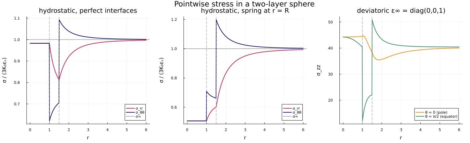
Figure 2 — a meridian map of the norm of the stress deviator
The deviatoric part of the uniaxial loading breaks the spherical symmetry, so the field is genuinely two-dimensional. A meridian slice
"Norm of the stress deviator, `σ_d = √(σᵈ:σᵈ)`."
deviatoric_norm(σ) = norm(σ - (tr(σ) / 3) * TensISO{3}(1.0))

xs = range(-2.6Rₛ, 2.6Rₛ; length = 220)
zs = range(-2.6Rₛ, 2.6Rₛ; length = 220)
σd_map = [
    let r = hypot(x, z)
        r < 1.0e-9 ? deviatoric_norm(local_flux(sol, [0.0, 0.0, 0.0], ε∞_uni)) :
            deviatoric_norm(local_flux(sol, [x, 0.0, z], ε∞_uni))
    end
        for z in zs, x in xs
]

fig2 = heatmap(
    xs, zs, σd_map;
    aspect_ratio = 1, c = :viridis, xlabel = "x", ylabel = "z",
    title = "σ_d = √(σᵈ:σᵈ), ε∞ = e₃⊗e₃",
    size = (620, 560), right_margin = 6Plots.mm
)
let θ = range(0, 2π; length = 400)
    plot!(fig2, R .* cos.(θ), R .* sin.(θ); lw = 1.5, color = :white, label = "")
    plot!(fig2, Rₛ .* cos.(θ), Rₛ .* sin.(θ); lw = 1.5, color = :white, ls = :dash, label = "")
end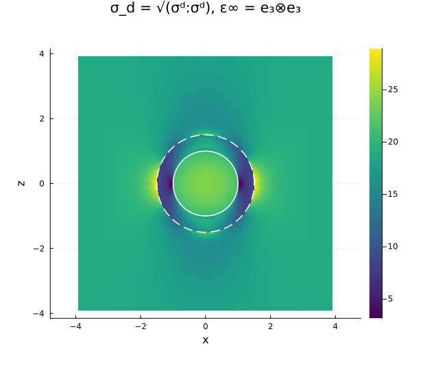
The pointwise field reproduces the layer averages
Averaging shell_concentration exposes that identity from the same cached amplitudes, so the two routes cannot drift apart.
println("\nlayer   α_k (pointwise)   α_k (averaged)   β_k (pointwise)   β_k (averaged)")
for k in 1:layer_count(sphere)
    αp, βp = shell_concentration(sol, k)
    A = gradient_gradient_concentration(sphere, C₀; layer = k)
    αa, βa = TensND.get_data(A)
    @printf "  %d      %14.10f   %14.10f   %14.10f   %14.10f\n" k αp αa βp βa
end
layer   α_k (pointwise)   α_k (averaged)   β_k (pointwise)   β_k (averaged)
  1        0.4423425706     0.4423425706     0.3273866458     0.3273866458
  2        1.6672912277     1.6672912277     1.6430810955     1.6430810955
The pointwise and averaged columns coincide layer by layer, both being read from the same amplitudes of the recurrence.
Where to go next
A sphere keeps every layer concentric and every field a function of the radius and of one angle. The n-layer confocal spheroid: geometry and effective conductivity gives up that symmetry for a nest of confocal spheroids, treated first in conduction, where the equivalent particle comes out of a harmonic series. The core, shell and matrix used above form the three-phase model of an aggregate and its interfacial transition zone, whose effect on the stiffness of a concrete is measured in The interfacial transition zone in concrete.
This page was generated using Literate.jl.