Levin's theorem: free strains and prestresses

Before this page

Homogenization schemes, where the strain and stress concentration tensors of an estimate are defined, and any of the scheme pages of this chapter, each of which ends with the concentration tensors of its estimate.

The schemes of this chapter estimate the response of a composite to a macroscopic strain alone. The phases of a real material often carry, in addition, a strain that owes nothing to the stress — a thermal dilation, a hydric or chemical swelling — or a stress that owes nothing to the strain, such as the pressure of a fluid filling the pores. The macroscopic law then acquires an additional term, and the theorem of Levin (1967), translated into English the same year (Levin, 1967), states that this term follows from the concentration tensors already computed, without any new problem to solve. Its consequences for thermal expansion were drawn by Rosen and Hashin (1970) for two anisotropic phases, the relations between the eigenstrains of the phases and their concentration tensors are developed for multiphase media by Dvorak and Benveniste (1992).

1. Setting

Each phase of the representative volume element obeys a linear elastic law with a uniform eigenstrain , or equivalently a uniform prestress ,

the stiffness having the major symmetry. The second form remains meaningful for a phase without stiffness, such as a pore filled with a fluid at pressure , where   and    . The local problem being linear in the pair , the macroscopic law is affine,

which defines the macroscopic prestress , the stress under a vanishing macroscopic strain, and the macroscopic free strain , the strain under a vanishing macroscopic stress. The concentration tensors are those of the problem without eigenstrain: the fields and give the local strain    under a macroscopic strain and the local stress    under a macroscopic stress, and their averages over phase are   and  . The fields and equal and in phase .

2. Statement

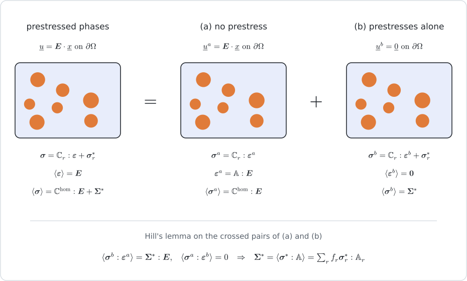
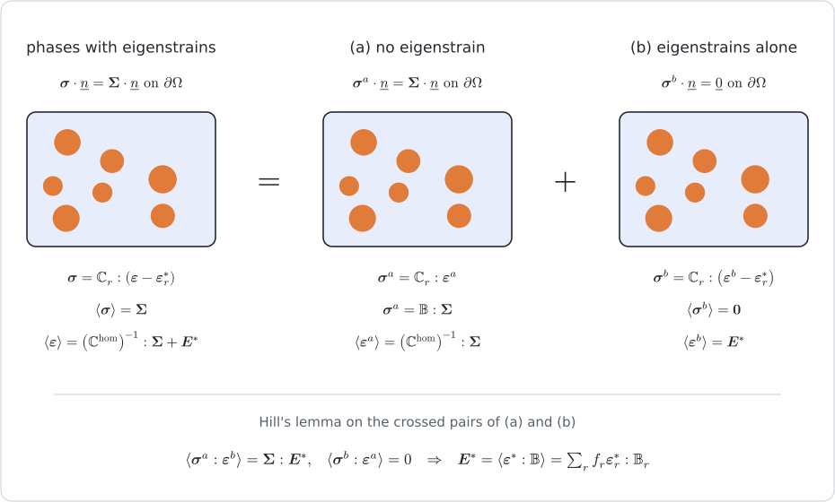
The macroscopic prestress and free strain are

the averages holding whatever the fields and , and the sums being their value for fields uniform in each phase. The second-order tensor contracts the first pair of indices of the fourth-order one,    . The concentration tensors have the minor symmetries but not the major one, so the order of the factors matters.

3. Proof

The local laws being linear, the problem with prestresses under a macroscopic strain is the sum of two problems posed on the same volume element under uniform strain boundary conditions (figure above). In problem (a) there is no prestress and the macroscopic strain is , so that    and   . In problem (b) the phases carry their prestresses and the macroscopic strain vanishes, so that   and  . Each stress field is in equilibrium and each strain field is compatible, so that Hill's lemma (Hill, 1963) applies to the two crossed pairs:

Pointwise, the major symmetry of the local stiffness yields           , whose average is

for every , so that   . Only the symmetry of the local stiffness was used, so that this holds for a phase without stiffness as well. For a prestress uniform in each phase, the average splits over the phases,        , which is the first statement.

The second statement follows from the dual decomposition, under uniform stress boundary conditions (figure above), when every phase has a stiffness and hence a compliance . In problem (a) there is no eigenstrain and the macroscopic stress is , so that    and   . In problem (b) the phases carry their eigenstrains and the macroscopic stress vanishes, so that   and  . Hill's lemma now gives

and, the compliance having the major symmetry too, pointwise     yields      , whose average is

for every , so that   . For an eigenstrain uniform in each phase,     , which is the second statement.

The two statements agree. The volume element being representative, a macroscopic strain and the macroscopic stress   produce the same fields, so that       at every point, and    . Substituting      in the first,

the last equality using the major symmetry of : it is the relation between the macroscopic prestress and the free strain of the setting.

4. With an estimate

A scheme provides estimates of and rather than the exact phase averages, and the theorem applied to them yields the estimate of and consistent with the scheme. The two forms of §2 remain equivalent as long as the estimate of keeps the major symmetry, on which the proof of the second one rests. A Mori–Tanaka estimate with inclusions of different shapes or orientations can lose it, and the two forms then give two different estimates; the package evaluates each one as stated, from for the prestress and from for the free strain.

Two phases

With two phases the averages      and        determine both stress concentration tensors, provided   is invertible:       and     . The free strain therefore depends on the effective compliance alone,

The derivation uses nothing but the two averages, which every estimate of the package satisfies: whatever the scheme, its estimate of the free strain of a two-phase material is this function of its estimate of . For two isotropic phases of bulk moduli , and thermal expansion coefficients , , under a temperature rise , the eigenstrains are    . Since    for the deviatoric projector and      , the thermal expansion tensor   is

which reduces to        when the effective compliance is isotropic,   .

5. Saturated pores and cracks: the Biot tensor

A fluid at pressure filling the pores loads them with the prestress  , and the macroscopic law takes the drained form      of Poromechanics, with the Biot tensor defined by    . A crack family filled by the same fluid contributes as well. Its volume fraction vanishes while the strain carried by its openings remains finite, so that the product   tends to  , the crack density times the concentration tensor per unit density defined in Homogenization schemes. Only the traction   on its faces enters the contraction, since the opening is a displacement jump across them. The first statement of §2 thus gives

When the solid is a single homogeneous phase , the two averages provide a shortcut: neither pores nor cracks carry stress, so that    , and the strain average then gives       , whence the classical      evaluated by biot_tensor. With several solid phases the shortcut is lost, and the theorem in the form above is the general route.

6. Conduction

The proof uses neither the order of the tensors nor the physics, only the symmetry of the local law and Hill's lemma, both of which hold in conduction with the dictionary of Extension to conductivity: the gradient for the strain, the opposite of the flux for the stress, vectors for the second-order tensors. A phase conducting no flux under the gradient , its eigengradient,

gives the composite the law           , with

where maps the macroscopic gradient onto the mean gradient of the phase and the macroscopic flux onto its mean flux. For two phases the free gradient again depends on the effective tensor alone,        . Such terms arise when a transport law carries, besides the gradient, a driving force that is uniform in each phase.

7. In the package

concentration_tensors returns the concentration tensors of every phase under a scheme, and the theorem is applied by levin_preflux and levin_free_gradient, which take the prestress or the eigenstrain of each loaded phase:

ct = concentration_tensors(rve, MoriTanaka(:M), :C)
𝟏 = TensISO{3}(1.0)
α_hom = levin_free_gradient(ct, Dict(:M => α_M * 𝟏, :I => α_I * 𝟏))
B = -levin_preflux(ct, Dict(:P => -𝟏, :cracks => -𝟏))

A crack family is accepted as a prestressed phase, with its density as weight, and refused as an eigenstrained one, since it holds no material. The same two functions serve conduction: they take vectors and the concentration tensors of a conduction estimate. In elasticity they also answer to levin_free_strain and levin_prestress, which refuse a conduction estimate:

ct_K = concentration_tensors(rve, MoriTanaka(:M), :K)
G = levin_free_gradient(ct_K, Dict(:M => g_M, :I => g_I))   # g_M = Tens([0.0, 0.0, 1.0]), …

Where to go next

The tutorial Thermal expansion and Biot tensor applies the theorem to a two-phase composite and to a porous solid, numerically and in closed form. The next chapter keeps every scheme and changes the physics: Extension to conductivity states the dictionary through which the order-2 transport problem reuses the whole chain.