
The n-layer confocal spheroid: geometry and effective conductivity
The whole page as one script
Every block of this page, in order, is scripts/32_spheroid_effective_conductivity.jl. From a clone of the repository, julia --project=docs -e 'using Pkg; Pkg.instantiate()' once, then julia scripts/32_spheroid_effective_conductivity.jl, runs it end to end.
Before this page
The tutorials n-layer sphere: volume-averaged concentration tensors, the spherical case of the composite inclusion treated here, and Transport properties, for the conduction problem it is solved in; the theory page Layered spheroid — confocal harmonic series derives the series evaluated below.
Every RVE phase seen so far has been a single ellipsoid or a layered sphere. LayeredSpheroid is an N-layer confocal spheroidal composite inclusion for conduction (thermal, electric, Darcy), following Barthélémy and Bignonnet (2020). It plugs into the same RVE / homogenize workflow as every other phase.
This page covers the geometry, the API, and the two effective quantities it produces: the effective conductivity of a composite reinforced by such particles, and the equivalent particle that reproduces it. What an imperfect interface does to the local fields is the subject of the companion page; the confocal-harmonic series behind all of it is on the theory page.
Conduction only
Unlike LayeredSphere, LayeredSpheroid has no elastic counterpart — the harmonic decomposition it relies on is specific to the scalar Laplace equation.
using MeanFieldHomogenization
using MeanFieldHomogenization.LayeredSpheroids: spheroid_ba_ratios, coupling_matrices
using TensND
using LinearAlgebra
using Printf
using Plots
gr()

default(; left_margin = 5Plots.mm, bottom_margin = 5Plots.mm)
Building a spheroid
A spheroid is specified by its per-layer axis (revolution) and disk (transverse) semi-axes — ascending, and confocal, i.e. axis² - disk² constant across layers up to sign.
K1 = TensISO{3}(20.0)      # inclusion conductivity
K0 = TensISO{3}(2.0)       # matrix conductivity

s = LayeredSpheroid((3.0,), (1.0,), (K1,))   # prolate, aspect ratio ϖ = 3
LayeredSpheroid{Float64} (1 layer(s), prolate, focal = 2.8284271247461903)With a single layer and a perfect interface, LayeredSpheroid must reduce exactly to the classical Eshelby result for a homogeneous spheroidal inclusion. This is the first regression test in test/LayeredSpheroids/test_conductivity.jl, and a good way to see that the machinery is anchored:
A_layered = gradient_gradient_concentration(s, K1, K0)

ell = Spheroid(3.0)                        # equivalent homogeneous Ellipsoid
P = hill_tensor(ell, K0)
A_classic = inv(TensISO{3}(1.0) + P ⋅ (K1 - K0))

A_layered ≈ A_classictrueSpheroid(ϖ)'s revolution axis is ê₁ for a prolate spheroid (aspect ratio \omega > 1) and ê₃ for an oblate one (\omega < 1); LayeredSpheroid's own default axis is ê₃, overridable with the axis keyword — pass axis = (1.0, 0.0, 0.0) when comparing against a prolate Spheroid, as above.
Imperfect interfaces
LayeredSpheroid reuses LayeredSphere's interface types: KapitzaInterface(ρ), a temperature-jump resistance ("LC", low-conducting), and SurfaceConductiveInterface(kₛ), a flux-jump surface conductance ("HC", highly-conducting), on top of the default PerfectInterface. An exact limit anchors them: an infinitely resistive interface must behave like a fully insulated core.
s_lc = LayeredSpheroid((3.0,), (1.0,), (K1,); interfaces = (KapitzaInterface(1.0e10),))
s_insulated = LayeredSpheroid((3.0,), (1.0,), (TensISO{3}(1.0e-12),))

gradient_gradient_concentration(s_lc, K1, K0) ≈ gradient_gradient_concentration(s_insulated, TensISO{3}(1.0e-12), K0)trueMultiple layers
Extend both semi-axis tuples (ascending, confocal) and the per-layer conductivity / interface tuples:
focal2 = 3.0^2 - 1.0^2                       # shared focal distance², outer layer
a_in = 2.9
b_in = sqrt(a_in^2 - focal2)                 # confocal inner layer

s2 = LayeredSpheroid(
    (a_in, 3.0), (b_in, 1.0), (TensISO{3}(5.0), K1);
    interfaces = (KapitzaInterface(0.1), PerfectInterface()),
)
layer_volume_fraction(s2, 1), layer_volume_fraction(s2, 2)
(0.39633333333333415, 0.6036666666666658)The convenience constructor layered_spheroid_from_fractions builds the confocal parameters from an outer aspect ratio, an outer size, and target volume fractions:
s3 = layered_spheroid_from_fractions(3.0, 3.0, (0.3, 0.7), (TensISO{3}(5.0), K1))
layer_volume_fraction(s3, 1), layer_volume_fraction(s3, 2)
(0.3000000000000018, 0.6999999999999982)In an RVE
LayeredSpheroid is a first-class phase geometry. It carries no Hill tensor (is_homogeneous_inclusion(s) == false), so it plugs into the schemes through its own volume-averaged concentration tensors instead. The declared phase property is accepted for signature compatibility but ignored — the real moduli live in the layers.
rve = RVE()
add_phase!(rve, :M, Ellipsoid(1.0, 1.0, 1.0), Dict(:K => K0); fraction = :rest)
add_phase!(rve, :I, s, Dict(:K => K1); fraction = 0.15)

get_array(homogenize(rve, MoriTanaka(), :K))
3×3 Matrix{Float64}:
2.61236 0.0 0.0
0.0 2.61236 0.0
0.0 0.0 3.4741Effective conductivity vs. the interface parameter
The benchmark configuration of Kushch et al. (2015): aligned prolate particles at volume fraction 0.5, conductivity contrast
The point of the sweep is the equivalent-particle theorem: the full confocal series solution of the imperfect-interface spheroid is homogenization-equivalent to a single homogeneous, perfectly-bonded ellipsoid carrying the anisotropic conductivity
where
const EC_KM = 1.0
const EC_K1 = 1.0e3
const EC_FRAC = 0.5
const EC_N = 5
const EC_AXIS = (1.0, 0.0, 0.0)
const EC_KINC = TensISO{3}(EC_K1)
const EC_KMAT = TensISO{3}(EC_KM)

_ec_particle(ϖ, ρ; N = EC_N) = LayeredSpheroid(
    (ϖ,), (1.0,), (EC_KINC,);
    interfaces = (MeanFieldHomogenization.KapitzaInterface(ρ),), Nseries = N, axis = EC_AXIS,
)

function _ec_series(ϖ, ρ, scheme)
    rve = RVE()
    add_phase!(rve, :M, Ellipsoid(1.0, 1.0, 1.0), Dict(:K => EC_KMAT); fraction = :rest)
    add_phase!(rve, :I, _ec_particle(ϖ, ρ), Dict(:K => EC_KINC); fraction = EC_FRAC)
    return homogenize(rve, scheme, :K)[1, 1]
end

function _ec_equiv(ϖ, ρ, scheme)
    p = _ec_particle(ϖ, ρ)
    A = gradient_gradient_concentration(p, EC_KINC, EC_KMAT)
    B = flux_gradient_concentration(p, EC_KINC, EC_KMAT)
    Keq = TensND.TensTI{2}(B[2, 2] / A[2, 2], B[1, 1] / A[1, 1], EC_AXIS)
    rve = RVE()
    add_phase!(rve, :M, Ellipsoid(1.0, 1.0, 1.0), Dict(:K => EC_KMAT); fraction = :rest)
    add_phase!(rve, :I, Ellipsoid(ϖ, 1.0, 1.0), Dict(:K => Keq); fraction = EC_FRAC)
    return homogenize(rve, scheme, :K)[1, 1]
end

const EC_H = exp10.(range(-2, 3; length = 60))     # h̃ = kₘ·b/ρ, b = 1
const EC_OMEGAS = (3.0, 10.0)
const EC_SCHEMES = (MoriTanaka(), Dilute())
const EC_NAMES = ("Mori–Tanaka", "Dilute")

ec_series = Dict{Tuple{Float64, Int}, Vector{Float64}}()
ec_equiv = Dict{Tuple{Float64, Int}, Vector{Float64}}()
ec_gap = 0.0
for ϖ in EC_OMEGAS, (si, sch) in enumerate(EC_SCHEMES)
    vs = [_ec_series(ϖ, EC_KM / h, sch) for h in EC_H]
    ve = [_ec_equiv(ϖ, EC_KM / h, sch) for h in EC_H]
    ec_series[(ϖ, si)] = vs
    ec_equiv[(ϖ, si)] = ve
    global ec_gap = max(ec_gap, maximum(abs.(vs .- ve) ./ abs.(vs)))
end

println("Imperfect-interface sweep — c = $EC_FRAC, k₁/kₘ = $EC_K1")
println("─"^70)
@printf "Largest relative gap |k_series − k_equiv| / |k_series| over the whole sweep\n"
@printf "(both schemes, both aspect ratios): %.2e\n" ec_gap
println("→ the layered spheroid and its equivalent ellipsoid homogenize identically.")
println()

p_eff = plot(
    xscale = :log10, xlabel = "h̃ = kₘ·b / ρ", ylabel = "k₁₁ᵉᶠᶠ / kₘ",
    title = "Effective axial conductivity vs. Kapitza interface parameter",
    legend = :topleft, size = (860, 560),
)
for (i, ϖ) in enumerate(EC_OMEGAS), (si, _) in enumerate(EC_SCHEMES)
    plot!(
        p_eff, EC_H, ec_series[(ϖ, si)] ./ EC_KM;
        label = "series, ϖ=$(round(Int, ϖ)), $(EC_NAMES[si])",
        color = (:steelblue, :darkorange)[i], linestyle = (:solid, :dash)[si], lw = 2,
    )
    scatter!(
        p_eff, EC_H[1:4:end], ec_equiv[(ϖ, si)][1:4:end] ./ EC_KM;
        label = "equivalent inclusion, ϖ=$(round(Int, ϖ)), $(EC_NAMES[si])",
        color = (:steelblue, :darkorange)[i], markershape = :circle, markersize = 4,
        markerstrokewidth = 1, markeralpha = 0.0,
        markerstrokecolor = (:steelblue, :darkorange)[i],
    )
end
p_eff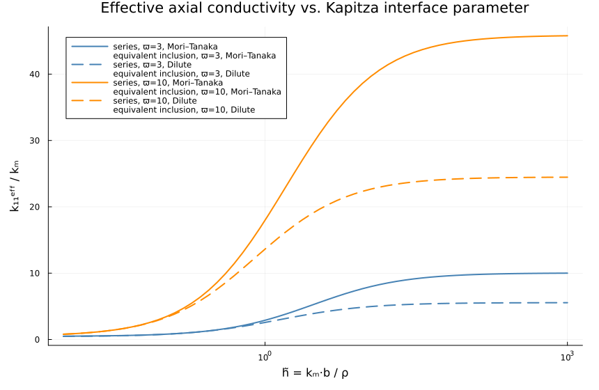
The equivalent particle itself
Here it is traced directly from the confocal transfer-matrix solution, at fixed physical size, against the aspect ratio.
const EQ_KM = TensISO{3}(1.0)
const EQ_KINC = TensISO{3}(10.0)
const EQ_A = 1.0                                   # fixed physical axis semi-axis
const EQ_RHOS = (0.0, 0.05, 0.2, 1.0)
const EQ_OMEGAS = exp10.(range(-0.9, 0.9; length = 50))

function _eq_keq(ϖ, ρ)
    ϖ ≈ 1 && return (NaN, NaN)
    p = LayeredSpheroid(
        (EQ_A,), (EQ_A / ϖ,), (EQ_KINC,);
        interfaces = (MeanFieldHomogenization.KapitzaInterface(ρ),), Nseries = 6,
    )
    A = gradient_gradient_concentration(p, EQ_KINC, EQ_KM)
    B = flux_gradient_concentration(p, EQ_KINC, EQ_KM)
    return real(B[1, 1] / A[1, 1]), real(B[3, 3] / A[3, 3])
end

p_keq = plot(
    xscale = :log10, xlabel = "aspect ratio ϖ", ylabel = "kᵉq / kₘ",
    title = "Equivalent particle conductivity (fixed size, Kapitza interface)",
    legend = :best, size = (860, 520),
)
for (i, ρ) in enumerate(EQ_RHOS)
    vals = [_eq_keq(ϖ, ρ) for ϖ in EQ_OMEGAS]
    plot!(p_keq, EQ_OMEGAS, first.(vals); label = "transverse, ρ=$ρ", lw = 2, color = i)
    plot!(p_keq, EQ_OMEGAS, last.(vals); label = "axial, ρ=$ρ", lw = 2, ls = :dash, color = i)
end
hline!(p_keq, [10.0]; color = :grey, ls = :dot, label = "bare inclusion (ρ = 0 limit)")
p_keq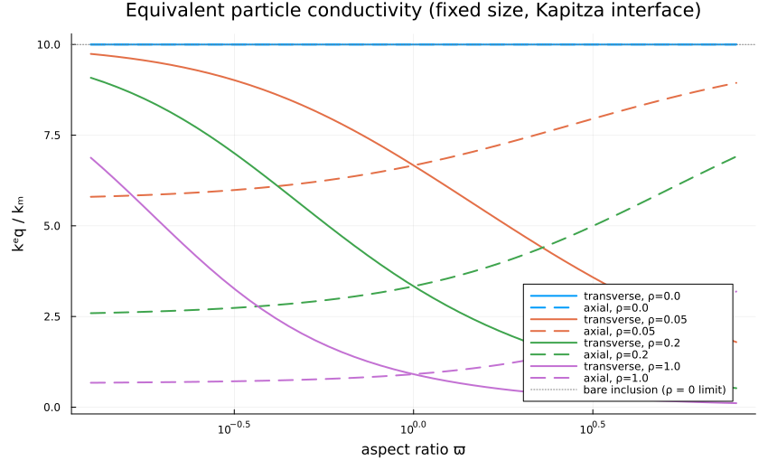
Numerical note: series truncation, and why quadrature
The confocal solution is a truncated harmonic series. How many terms
The convergence study below uses a single-layer prolate spheroid with an insulating core and a unit HC interface. For each aspect ratio, the relative change of the leading coefficients between
const CV_KM = TensISO{3}(1.0)
const CV_KCORE = TensISO{3}(0.0)
const CV_OMEGAS = (1.1, 2.0, 1.0e1, 1.0e2, 1.0e3, 1.0e4)
const CV_NMAX = 15

function _cv_sequence(ϖ)
    mk(N) = LayeredSpheroid(
        (ϖ,), (1.0,), (CV_KCORE,);
        interfaces = (MeanFieldHomogenization.SurfaceConductiveInterface(1.0),),
        Nseries = N, axis = (1.0, 0.0, 0.0),
    )
    return [spheroid_ba_ratios(mk(N), CV_KM) for N in 2:CV_NMAX]
end

cv_a = Dict{Float64, Vector{Float64}}()
cv_t = Dict{Float64, Vector{Float64}}()
for ϖ in CV_OMEGAS
    seq = _cv_sequence(ϖ)
    ba = first.(seq); bt = last.(seq)
    cv_a[ϖ] = [abs((ba[i] - ba[i - 1]) / ba[i - 1]) for i in 2:length(ba)]
    cv_t[ϖ] = [abs((bt[i] - bt[i - 1]) / bt[i - 1]) for i in 2:length(bt)]
end

println("Convergence of the leading coefficients vs 𝒩 (insulating core, unit HC interface)")
println("─"^78)
for ϖ in CV_OMEGAS
    @printf "ϖ=%8.1e   rel.diff @ 𝒩=5: axial=%.2e trans=%.2e   @ 𝒩=10: axial=%.2e trans=%.2e\n" ϖ cv_a[ϖ][4] cv_t[ϖ][4] cv_a[ϖ][9] cv_t[ϖ][9]
end
println()
Convergence of the leading coefficients vs 𝒩 (insulating core, unit HC interface)
──────────────────────────────────────────────────────────────────────────────
ϖ= 1.1e+00 rel.diff @ 𝒩=5: axial=3.96e-16 trans=2.28e-16 @ 𝒩=10: axial=5.94e-16 trans=0.00e+00
ϖ= 2.0e+00 rel.diff @ 𝒩=5: axial=1.15e-08 trans=1.83e-08 @ 𝒩=10: axial=1.64e-14 trans=2.69e-14
ϖ= 1.0e+01 rel.diff @ 𝒩=5: axial=5.72e-05 trans=8.05e-05 @ 𝒩=10: axial=3.30e-07 trans=5.50e-07
ϖ= 1.0e+02 rel.diff @ 𝒩=5: axial=7.31e-05 trans=1.45e-04 @ 𝒩=10: axial=1.44e-05 trans=3.02e-06
ϖ= 1.0e+03 rel.diff @ 𝒩=5: axial=1.77e-06 trans=1.45e-04 @ 𝒩=10: axial=7.98e-07 trans=3.03e-06
ϖ= 1.0e+04 rel.diff @ 𝒩=5: axial=2.66e-08 trans=1.45e-04 @ 𝒩=10: axial=1.29e-08 trans=3.03e-06The original algorithm expands Legendre products into monomials, whose coefficients grow like MeanFieldHomogenization integrates the paper's own integral definitions by Gauss quadrature instead and never forms that ill-conditioned sum. Both must still agree, since they compute the same integrals two ways:
for N in (8, 12, 16)
    Iq, = coupling_matrices(3.0, N; method = :quadrature)
    Is, = coupling_matrices(3.0, N; method = :series)
    err = maximum(abs.(Iq .- Is)) / maximum(abs.(Is))
    @printf "𝒩=%2d  (series needs %2d digits)  max rel. diff = %.2e\n" N round(Int, 0.8 * (2N - 1)) err
end
println()

p_cv_a = plot(
    xlabel = "N (truncation order)", ylabel = "rel. change, axial",
    yscale = :log10, ylims = (1.0e-16, 1.0e-1), title = "Axial", legend = :topright,
)
p_cv_t = plot(
    xlabel = "N (truncation order)", ylabel = "rel. change, transverse",
    yscale = :log10, ylims = (1.0e-16, 1.0e-1), title = "Transverse", legend = :topright,
)
markers = (:circle, :diamond, :utriangle, :square, :star5, :cross)
for (i, ϖ) in enumerate(CV_OMEGAS)
    lbl = ϖ ≥ 10 ? @sprintf("ϖ=%.0e", ϖ) : @sprintf("ϖ=%.1f", ϖ)
    scatter!(p_cv_a, 3:CV_NMAX, max.(cv_a[ϖ], 1.0e-17); label = lbl, marker = markers[i], ms = 4)
    scatter!(p_cv_t, 3:CV_NMAX, max.(cv_t[ϖ], 1.0e-17); label = lbl, marker = markers[i], ms = 4)
end
p_cv = plot(p_cv_a, p_cv_t; layout = (1, 2), left_margin = 8Plots.mm, bottom_margin = 8Plots.mm, size = (1200, 500))
p_cv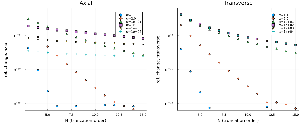
Each marker of the last figure is the relative change of a leading coefficient when one term is added to the series, so the slope of a sequence measures how many terms its aspect ratio needs.
Where to go next
The effective conductivity measures how much an imperfect interface matters, not what it does. Imperfect interfaces: what they do to the local fields reconstructs the temperature and the flux pointwise around a Kapitza and a highly conducting interface, on the same confocal solution. The constructor of LayeredSpheroid, its interface types and its truncation keyword are documented in Layered inclusions of the manual.
This page was generated using Literate.jl.