Nonlinear poroelasticity of a cracked rock

The whole page as one script

Every block of this page, in order, is scripts/material_laws/16_closing_cracks.jl. From a clone of the repository, julia --project=docs -e 'using Pkg; Pkg.instantiate()' once, then julia scripts/material_laws/16_closing_cracks.jl, runs it end to end.

A rock that contains microcracks is soft under a small confinement and stiffens as the confinement grows, because its cracks close one after the other. The same mechanism makes its Biot coefficient decrease with the confinement: a closed crack no longer stores fluid, and no longer transmits the pore pressure to the solid. Walsh (1965) explained the nonlinear compressibility of rocks in this way. Deudé et al. (2002) put it in a micromechanical setting of nonlinear poroelasticity. This page derives the law that MeanFieldHomogenization builds from the linear poroelasticity of the cracked solid. The example below runs it.

The linear poroelastic solid at given open cracks

The rock is an elastic solid of stiffness , containing families of penny-shaped cracks that an incompressible fluid saturates. Family has the normal and, when all its cracks are open, the density . As long as the set of open cracks does not change, the rock is a linear poroelastic solid (Coussy, 2004). Its drained stiffness is that of the solid with the open cracks, from any scheme of the package. Its Biot tensor and Biot modulus follow from and (see Poromechanics):

being the compliance of the solid and the porosity that the fluid occupies, here the volume of the cracks, small for thin cracks. The cracks make softer and larger.

What closes the cracks

The loading of the saturated rock is the macroscopic stress and the pore pressure . It splits into two problems. In the first, the pore pressure acts everywhere: on the faces of the cracks and in the pores, and, through a stress  , on the solid. This field is uniform; it carries no concentration at the tips of the cracks and cannot open or close them. The second problem is that of the dry rock under the Terzaghi effective stress

and that problem alone opens and closes the cracks. This argument, which the fractured-rock material of Barthélémy and Daniel (2011) already rests on, holds whatever the stiffness of the solid. It is the effective stress of the closure. The deformation obeys another one, the Biot effective stress   , as the rate equations below show: a pore pressure reopens the cracks fully, but deforms the rock only through .

A flat crack of aspect ratio closes when the compressive normal traction on its plane reaches a stress proportional to (and to the stiffness of the solid). A family is a population of cracks of various aspect ratios, so that the thinner ones close first. Under the normal effective traction    , a fraction of its cracks remains open, and its open density is  . The fraction depends on the distribution of the aspect ratios; an exponential distribution of the closure stresses, of mean , gives

ExponentialClosure: every crack is open in tension, and a fraction of them remains open under a compression . A closed crack transmits both normal and shear tractions, as in the fractured-rock material.

The rate equations

During a small increment of the loading, the cracks open at that moment behave as in the linear solid, and a crack that closes stops contributing to the next increments. The rates are therefore those of the linear solid with the current open densities:

being the change of fluid content. The first equation is      rewritten for the effective stress. The moduli depend on the state only through the open densities, hence through the normal effective tractions.

The law is hypoelastic: the moduli are tangent moduli, and in general they are not the second derivatives of a potential. The crack compliance mixes normal and shear parts, while the closure depends on the normal traction only. The response is therefore obtained by integrating the rates along the loading path, not by a formula of the current state.

The law in MaterialLaws

ClosingCrackPoroelasticity builds a ResidualLaw with two gradients, the strain and the pore pressure, and their two fluxes, the stress and the fluid content. Its internal variables are the effective stress and the fluid content . A step integrates the rates by the backward Euler scheme, with the moduli at the end of the step:

The stress is    . The scheme is first order: halving the steps halves the error. The consistent tangent follows from the implicit-function theorem and contains the variation of the moduli with the effective stress during the step; every block of it, between the strain and the pressure, the stress and the fluid content, is computed.

Scope

families	oriented, each seeing one normal traction; a family symmetrized over all orientations is refused, since its cracks see different tractions (several oriented families sample the orientations instead)
closure	any open fraction , one per family; closed cracks are welded (no sliding, no friction, no hysteresis)
fluid	incompressible, as in the fractured-rock material; the porosity is held at its given value while the cracks close
not covered	the permeability of the cracks; the opening of the cracks beyond their initial aperture under tension

Example: a cracked rock under confinement

This example runs the nonlinear poroelastic law of a cracked rock: a rock whose microcracks close as it is confined, so that its stiffness rises and its Biot coefficient falls. It then shows the two roles of the pore pressure, which reopens the cracks through the Terzaghi effective stress but deforms the rock through the Biot one.

The rock

A solid of bulk modulus 40 GPa and shear modulus 25 GPa holds three families of microcracks, normal to the three axes, each of density 0.1. Three orthogonal families are the simplest sampling of the orientations that keeps the rock symmetric under a hydrostatic loading. Their closure stresses are distributed exponentially, with a mean of 20 MPa.

using MeanFieldHomogenization, TensND, Plots

C_s = TensISO{3}(3 * 40e3, 2 * 25e3)                                  # MPa
rve = RVE()
add_phase!(rve, :M, Ellipsoid(1.0), Dict(:C => C_s); fraction = :rest)
add_phase!(rve, :F3, PennyCrack(1.0), Dict(:C => C_s); density = 0.1)                          # normal e₃
add_phase!(rve, :F1, PennyCrack(1.0; euler_angles = (π / 2, 0.0)), Dict(:C => C_s); density = 0.1)      # normal e₁
add_phase!(rve, :F2, PennyCrack(1.0; euler_angles = (π / 2, π / 2)), Dict(:C => C_s); density = 0.1)    # normal e₂
rock = ClosingCrackPoroelasticity(rve; closure = ExponentialClosure(20.0), porosity = 0.005)

code	theory
rve	the solid and its crack families, at their densities with every crack open
closure	the open fraction of a family under the normal effective traction
porosity	the porosity occupied by the fluid, which sets the Biot modulus

Drained confinement

The rock is confined to 80 MPa with the pore pressure held at zero, so that the effective stress is the total stress:

P_max = 80.0
confine = LoadingPath(range(0, 1; length = 41); σ11 = t -> -P_max * t, σ22 = t -> -P_max * t,
    σ33 = t -> -P_max * t, σ23 = 0, σ13 = 0, σ12 = 0, p = 0)
r = point_response(rock, confine)

The moduli at each state are read on the consistent tangent of a step that does not move. Its blocks are the drained stiffness and the Biot tensor . Their isotropic parts give the drained bulk modulus and the Biot coefficient :

function moduli(law, state)
    _, 𝕂, _ = point_update(law, state.g, state, 1.0)
    K = sum(𝕂[1:3, 1:3]) / 9                  # (1 : C : 1) / 9
    b = sum(𝕂[7, 1:3]) / 3                    # (1 : B) / 3
    return K, b
end
P = -r[:σ11]
Kb = [moduli(rock, st) for st in r.states]
p1 = plot(P, first.(Kb) / 1e3; lw = 2, label = "", xlabel = "confining pressure (MPa)",
    ylabel = "drained bulk modulus K (GPa)")
hline!(p1, [40.0]; ls = :dash, label = "solid without cracks")
p2 = plot(P, last.(Kb); lw = 2, label = "", xlabel = "confining pressure (MPa)", ylabel = "Biot coefficient b")
plot(p1, p2; layout = (1, 2), size = (760, 320), left_margin = 3Plots.mm, bottom_margin = 4Plots.mm)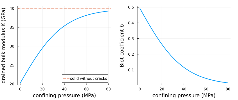

At zero confinement every crack is open: the rock has the linear moduli of the cracked solid. As the confinement grows the cracks close, the bulk modulus rises toward that of the solid and the Biot coefficient falls. The rise is fastest at low pressure, where the thinnest cracks close.

The pore pressure reopens the cracks

Starting from the confined state, the total stress is now held at 80 MPa and the pore pressure raised to 60 MPa. The effective stress falls to 20 MPa, and the cracks that the confinement had closed reopen:

times = vcat(range(0, 1; length = 41), range(1.025, 2; length = 40))
both = LoadingPath(times; σ11 = t -> -P_max * min(t, 1), σ22 = t -> -P_max * min(t, 1),
    σ33 = t -> -P_max * min(t, 1), σ23 = 0, σ13 = 0, σ12 = 0, p = t -> 60.0 * max(t - 1, 0))
r2 = point_response(rock, both)
reopen = 41:length(r2.t)
K2 = [moduli(rock, st)[1] for st in r2.states[reopen]]
p1 = plot(P, first.(Kb) / 1e3; lw = 2, label = "drained confinement",
    xlabel = "effective pressure −Σ′ (MPa)", ylabel = "drained bulk modulus K (GPa)", legend = :bottomright)
plot!(p1, -r2[:Σ′11][reopen], K2 / 1e3; lw = 2, ls = :dash, label = "pore pressure raised")
p2 = plot(P, 3 * r[:ε11] * 1e3; lw = 2, label = "drained confinement",
    xlabel = "effective pressure −Σ′ (MPa)", ylabel = "volume change (‰)", legend = :bottomleft)
plot!(p2, -r2[:Σ′11][reopen], 3 * r2[:ε11][reopen] * 1e3; lw = 2, ls = :dash, label = "pore pressure raised")
plot(p1, p2; layout = (1, 2), size = (760, 320), left_margin = 3Plots.mm, bottom_margin = 4Plots.mm)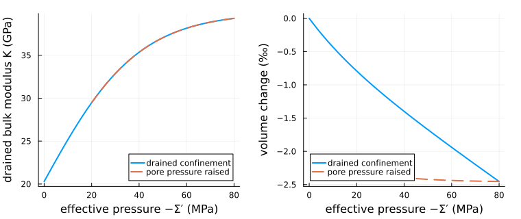

The two plots tell the two principles of the theory apart. The moduli are the same along both paths at the same effective pressure: the open cracks, hence the stiffness and the Biot tensor, depend on the Terzaghi effective stress alone. The deformation is not: raising the pore pressure recovers only part of the volume that the confinement took. The strain rate is    , and while most cracks are closed the Biot coefficient is small, so that the pore pressure acts on the deformation far less than on the cracks.

Checks

Every crack open: the linear cracked rock. Under a dilation no crack closes, and the law gives the moduli of the fractured-rock material FracturedPoroelasticRock with every family open:

fr = FracturedPoroelasticRock(rve, MoriTanaka(); ω₀ = (1e-3, 1e-3, 1e-3), porosity_ref = 0.005)
g = (ε = Mandel{Float64}(1e-4, 1e-4, 1e-4, 0, 0, 0), p = 0.0)
a = material_response(rock, g, initial_state(rock), 1.0).tangents.φp
b = material_response(fr, (ε = TensND.from_mandel(g.ε), p = g.p), initial_state(fr), 1.0).tangents.φp
a ≈ b

true

The tangent is consistent, every block of it:

check_material_interface(rock; verbose = false)

true

Going further

• Families symmetrized over all orientations are refused, since their cracks do not see one normal traction. More oriented families sample the orientations more finely.

• Each family may close in its own way: closure = (F1 = …, F2 = …, F3 = …), or any function of the normal traction.

• The law has two fields and runs in a coupled finite-element computation as the poroelastic laws of the finite-element coupling do.

---

This page was generated using Literate.jl.